Mortgage Bonds
A mortgage is a loan which is collateralized by real estate. Mortgages have two different ways of terminating:
- Prepayment: the borrower pays off the mortgage
- Default: the borrower can no longer make payments on the mortgage and the property is foreclosed upon by the bank. The bank ultimately takes possession of the house and sells it, often taking a loss on the mortgage.
Many mortgages can be pooled together and sold as bonds. The US mortgage bond market is one of the largest and most liquid markets in the world. For a mortgage bond:
- If all the loans prepay, the principal of the bond will be fully paid off.
- If all the loans default, the bond may lose principal.
A Simple Model of Prepayments and Defaults
Suppose that, each month, 2% of the balance prepays and 1% of the balance defaults. How much of the balance will ultimately default? Since $\frac{1}{3}$ of the balance is defaulting each period, $\frac{1}{3}$ of the balance will ultimately default.
Now suppose $x$% of the balance prepays and $y$% defaults each month. By a similar argument, $\frac{y}{x+y}$ of the balance will ultimately default.
A More Realistic Model of Prepayments and Defaults
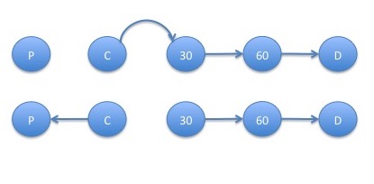
Every mathematical model is an idealization of reality. We now put a bit more realism into our model of mortgage prepayments and defaults. A borrower defaults on their mortgage after they have missed multiple payments. To make our model more realistic, we assume that a borrower is in default after missing 2 monthly payments. After missing 1 payment, the following possibilities exist for the next payment period:
- Catch-up: the borrower makes both the new payment and the previously missed payment becoming current on their mortgage
- Roll: the borrower makes only the new payment remaining 1 payment behind
- Miss another payment: the borrower makes no payment and goes into default
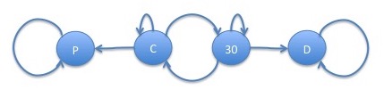
where:
- C represents the state in which the borrower is up to date (current) on their mortgage payments
- 30 represents the state in which the borrower is one monthly payment (30 days) behind on their mortgage payments
- P represents the state in which the borrower has paid off (prepayed) their mortgage
- D represents the state in which the borrower has defaulted on their mortgage
Similar to the last example, we would like to know, given the probabilities of transitioning between different states of the graph, what the probability of eventual default is. Near the beginning of the bond's life, all mortgages are in state $C$ so there will be no loans defaulting but some loans may be prepaying. Hence, using the previous rule, we would estimate the default probability as $0$. We would like a more accurate formula for this situation.
Let $p_{s_1,s_2}$ denote the probability of going from state $s_1$ to state $s_2$ which we assume is known (we discuss methods for estimating these probabilities later in this course). These probabilities are refered to as transition probabilities. For example, $p_{C,30}$ denotes the probability of going from $C$ to $30$. Furthermore, we introduce the unknown quantities $q_{s_1,s_2}$ for the probability that we eventually end up in $s_2$ starting in $s_1$. Note that every loan eventually ends up in either state P or state D. As a result, we have that $q_{s,P} + q_{s,D} = 1$ and so we need only solve for $q_{s,D}$.
Consider a loan in state $C$. There are $3$ possibilities:
- The loan stays in state $C$: the probability of this is $p_{C,C}$ and the probability that the loan subsequently ends up in state $D$ is $q_{C,D}$
- The loan moves to state $30$: the probability of this is $p_{C,30}$ and the probability that the loan subsequently ends up in state $D$ is $q_{30,D}$
- The loan moves to state $P$: the probability of this is $p_{C,P}$ and there is no probability that the loan subsequently ends up in state $D$
A Still More Realistic Model of Prepayments and Defaults
The laws applying to the default of mortgages in the United States are at a state level, with each state having its own peculiarities. In many states, a borrower must miss 3 payments before the lender is allowed to file a "Notice of Default". We now model this requirement. For simplicity, we will assume that a borrower is either able to make no payments, 1 payment or all payments when they are delinquent, which tend to be the common behaviors.
This model is represented by the following graph:
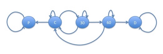
Since this model would involve a set of $3$ equations in $3$ unknowns which is starting to become unwieldy, we generalize the approach of the previous model using matrix algebra in the next section to show a computational approach to solving for the probability of eventual default.
Matrix Algebraic Calculation of Absorption Probabilities
The matrix of transition probabilities is given by: \[ P = \left(\begin{array}{ccccc} p_{P,P} & p_{P,C} & p_{P,30} & p_{P,60} & p_{P,D}\\ p_{C,P} & p_{C,C} & p_{C,30} & p_{C,60} & p_{C,D}\\ p_{30,P} & p_{30,C} & p_{30,30} & p_{30,60} & p_{30,D}\\ p_{60,P} & p_{60,C} & p_{60,30} & p_{60,60} & p_{60,D}\\ p_{D,P} & p_{D,C} & p_{D,30} & p_{D,60} & p_{D,D}\\ \end{array}\right) \] Note that many of these transition probabilities are $0$, since there is no arrow in the state diagram for them. Also, $p_{P,P}$ and $p_{D,D}$ are $1$ since they are the only outgoing arrows from these states, the probability of going from state $P$ or $D$ to itself is $1$. The states $P$ and $D$ are referred to as absorbing states. With the $0$'s and $1$'s, the $P$ matrix becomes: \[ P = \left(\begin{array}{ccccc} 1 & 0 & 0 & 0 & 0\\ p_{C,P} & p_{C,C} & p_{C,30} & 0 & 0\\ 0 & p_{30,C} & p_{30,30} & p_{30,60} & 0\\ 0 & p_{60,C} & 0 & p_{60,60} & p_{60,D}\\ 0 & 0 & 0 & 0 & 1\\ \end{array}\right) \] In order to demonstrate how to calculate absorption probabilities, that is, the probabilities of eventually ending in state $D$, we introduce the vector $q$: \[ q = \left(\begin{array}{c} q_{P,D}\\ q_{C,D}\\ q_{30,D}\\ q_{60,D}\\ q_{D,D}\\ \end{array}\right) \] Note that since state $D$ is absorbing, the probability of ending up in $D$ starting from $D$ is $1$. Similarly since state $P$ is absorbing, the probability of ending up in $D$ starting from $P$ is $0$. With the $0$'s and $1$'s, the $q$ vector becomes: \[ q = \left(\begin{array}{c} 0\\ q_{C,D}\\ q_{30,D}\\ q_{60,D}\\ 1\\ \end{array}\right) \] We now consider $q_{C,D}$. From $C$, we can transition to states $P$, $C$ and $30$. After transitioning to some state $s$, the probability of eventually ending in $D$ becomes $q_{s,D}$. Hence, and equation for $q_{C,D}$ is: \[ q_{C,D} = p_{C,P} q_{P,D} + p_{C,C} q_{C,D} + p_{C,30} q_{30,D}\\ \] In this case, $q_{P,D} = 0$ so the equation simplifies to: \[ q_{C,D} = p_{C,C} q_{C,D} + p_{C,30} q_{30,D}\\ \] In general, for some state $s$, the equation for $q_{s,D}$ is: \[ q_{s,D} = \sum_{s'} p_{s,s'} q_{s',D}\\ \] or, in matrix notation: \[ q = P q\\ \] Note that this is $n$ equations in $n$ unknowns, where $n$ is the number of states, in this case $5$. However, the top and bottom equation are redundant. The top equation is $q_{P,D} = p_{P,P}q_{P,D}$ which becomes $q_{P,D} = q_{P,D}$. The same holds for the bottom equation. Hence, we need $2$ additional equations to solve the system. The additional equations are $q_{P,D} = 0$ and $q_{D,D} = 1$ as already mentioned. Rearranging and putting the equations together yields the following set of equations: \[ \left(\begin{array}{cccc} 1 & 0 & 0 & 0 & 0\\ p_{C,P} & p_{C,C} - 1 & p_{C,30} & 0 & 0\\ 0 & p_{30,C} & p_{30,30} - 1 & p_{30,60} & 0\\ 0 & p_{60,C} & p_{60,30} & p_{60,60} - 1 & p_{60,D}\\ 0 & 0 & 0 & 0 & 1\\ \end{array}\right) q = \left(\begin{array}{c} 0\\ 0\\ 0\\ 0\\ 1\\ \end{array}\right)\\ \] This equation can be solved numerically by inverting the matrix on the left and multiplying by the vector on the right.
Graph Theoretic Calculation of Absorption Probabilities
There is another approach to deriving a formula for absorption probabilities involving graph theory, the branch of mathematics which studies graphs. We call one of the lines with an arrow on the end within a graph an edge. The following steps will derive a formula for the probability of being eventually absorbed into some state $D$:
- Find all graphs that can be formed by starting with this graph and removing enough of the edges such that:
- For any state $s'$, it is not possible to get from $s'$ back to $s'$ by traversing a sequence of edges (containing at least one edge) in the direction of the arrows.
- Every non-absorbing state has exactly one outgoing edge.
- For each of these graphs, find the product of the transition probabilities corresponding to the edges in the graph.
- For any state $s$:
- Find all graphs from step I above such that it is possible to get from $s$ to $D$ by traversing edges in the direction of the arrow.
- The absorption probability from state $s$ to $D$ is the sum of the products corresponding to state $s$ divided by the sum of the products corresponding to all graphs.
Example: Model of Prepayments and Defaults
The graphs with the listed properties are:
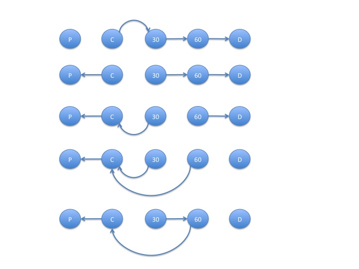
- The products of the transition probabilities corresponding to the edges in the graphs above are: \[ p_{C,30} p_{30,60} p_{60,D}\\ p_{C,P} p_{30,60} p_{60,D}\\ p_{C,P} p_{30,C} p_{60,D}\\ p_{C,P} p_{30,C} p_{60,C}\\ p_{C,P} p_{30,60} p_{60,C}\\ \]
- For state $C$:
The graphs such that it is possible to get from state $C$ to state $D$ are:
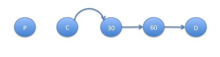
- The absorption probability from state $C$ to state $D$ is given by: \[ q_{C,D} = \frac{p_{C,30} p_{30,60} p_{60,D}}{p_{C,30} p_{30,60} p_{60,D} + p_{C,P} p_{30,60} p_{60,D} + p_{C,P} p_{30,C} p_{60,D} + p_{C,P} p_{30,C} p_{60,C} + p_{C,P} p_{30,60} p_{60,C}} \]
- For state $30$:
The graphs such that it is possible to get from state $30$ to state $D$ are:
- The absorption probability from state $30$ to state $D$ is: \[ q_{30,D} = \frac{p_{C,30} p_{30,60} p_{60,D} + p_{C,P}p_{30,60}p_{60,D}}{p_{C,30} p_{30,60} p_{60,D} + p_{C,P} p_{30,60} p_{60,D} + p_{C,P} p_{30,C} p_{60,D} + p_{C,P} p_{30,C} p_{60,C} + p_{C,P} p_{30,60} p_{60,C}} \]
Example: Birth Death Processes
Consider a stock which can go up or down by at most a single tick each period. This type of Markov chain is sometimes referred to as a birth death process, though this term refers to the continuous-time version of the process, from its origins in population biology. Suppose the stock starts at some price $S_0$. We invest in the stock but if the stock hits a level $L < S_0$, we cut our losses and sell. Also, if the stock hits a desired level $U>S_0$, we have made a sufficient amount and we exit the position. What is the probability that we hit $U$ before hitting $L$? We'll answer this question using the approach to calculating absorption probabilities just discussed.
Labeling each state with the number of ticks corresponding to the price, the graph for this Markov chain is:

For any state $i$, we will let $u_i$ be the probability that the stock moves up in the next step and $d_i$ the probability that it moves down. The stock will stay in the same place with the remaining probability, $1-u_i-d_i$. The calculation of absorption probabilities proceeds as follows:
Note that if we don't remove an edge from $i$ to $i+1$ in the graph, then the edge from $i+1$ to $i$ must be removed. This means that if the remaining edges are moving upwards at $i$, since each non-absorbing state must have an outgoing edge, they must move upwards from that point to the upper absorbing state $U$. Similarly, if the edge from $i-1$ to $i-2$ is present, the graph moves downwards from $i-1$ through the lower absorbing state $L$. Hence, the graph with the remaining edges moves downwards from some state $i$ and below and upwards from state $i+1$ and above. It looks something like this (where $i=L+3$:

- The products of the transition probabilities corresponding to the edges in the above graphs are, for each state $i$: \[ \prod_{j=L+1}^{i-1}d_j \times \prod_{j=i}^{U-1} u_j = d_{L+1} d_{L+2} \ldots d_{i-2} d_{i-1} u_i u_{i+1} \ldots u_{U-2} u_{U-1} \]
- For state $S_0$:
- The graphs such that it is possible to get from state $S_0$ to $U$ are the ones where the point at which the edges move upwards start from $i\leq S_0$.
- The absorption probability from state $S_0$ to state $U$ is: \[ q_{S_0,U} = \frac{\sum_{i=L+1}^{S_0} \prod_{j=L+1}^{i-1} d_j \times \prod_{j=i}^{U-1} u_j}{\sum_{i=L+1}^U \prod_{j=L+1}^{i-1} d_j \times \prod_{j=i}^{U-1} u_j} \]
The summation in the last formula is an example of a geometric series, that is, an infinite series in which each element is exponential in the index. This is an important result which will appear later in this course so we will take a few moments to show how it is solved. First, consider a simple geometric series which we label as $x$: \begin{eqnarray} x = \sum_{i=0}^\infty a^i \end{eqnarray} We now note that $x - ax = 1$: \begin{eqnarray} x - a x = \sum_{i=0}^\infty a^i - a\sum_{i=0}^\infty a^i = \sum_{i=0}^\infty a^i - \sum_{i=0}^\infty a^{i+1} = \sum_{i=0}^\infty a^i - \sum_{i=1}^\infty a^i = 1 \end{eqnarray} Hence, $x(1-a)=1$ or $x = \frac{1}{1-a}$ so: \begin{eqnarray} \sum_{i=0}^\infty a^i = \frac{1}{1-a} \end{eqnarray} Note that if $|a|\geq 1$, the geometric series does not converge to a finite value and so this formula is only valid for $|a|<1$.
Now we consider a truncated geometric series: \begin{eqnarray} \sum_{i=0}^{n-1} a^i \end{eqnarray} Note that this is the difference between the geometric series and a multiple of the geometric series: \begin{eqnarray} \sum_{i=0}^{n-1} a^i = \sum_{i=0}^\infty a^i - a^n \sum_{i=0}^\infty a^i = \frac{1}{1-a} - \frac{a^n}{1-a} = \frac{1 - a^n}{1 - a} \end{eqnarray}
Using this formula in (\ref{preruin}), we get: \begin{eqnarray} q_{S_0,U} = \frac{d^{-L-1}u^U\sum_{i=L+1}^{S_0} \left(\frac{d}{u}\right)^i}{d^{-L-1}u^U\sum_{i=L+1}^U \left(\frac{d}{u}\right)^i} = \frac{\frac{\left(\frac{d}{u}\right)^{L+1} - \left(\frac{d}{u}\right)^{S_0+1}}{1-\frac{d}{u}}}{\frac{\left(\frac{d}{u}\right)^{L+1} - \left(\frac{d}{u}\right)^{U+1}}{1-\frac{d}{u}}} = \frac{\left(\frac{d}{u}\right)^{L+1} - \left(\frac{d}{u}\right)^{S_0+1}}{\left(\frac{d}{u}\right)^{L+1} - \left(\frac{d}{u}\right)^{U+1}} = \frac{\left(\frac{d}{u}\right)^{S_0-L} - 1}{\left(\frac{d}{u}\right)^{U-L} - 1}\tag{2}\label{ruin} \end{eqnarray} using the formula for a truncated geometric series.
Note that there were mistakes on previous versions of this formula. It is important to find ways of checking your formulas. In this case, we can check the formula from the formula for default of the simple prepayment and default model. If the prepayment rate is $d$ and the default rate $u$ then the probability of default is $\frac{u}{u+d}$ whereas (\ref{ruin}) yields: \begin{eqnarray} \frac{\left(\frac{d}{u}\right)^{S_0-L} - 1}{\left(\frac{d}{u}\right)^{U-L} - 1} = \frac{\frac{d}{u} - 1}{\left(\frac{d}{u}\right)^2 - 1} = \frac{\frac{d}{u} - 1}{\left(\frac{d}{u}-1\right)\left(\frac{d}{u}+1\right)} = \frac{1}{\frac{d}{u}+1} = \frac{u}{d+u} \end{eqnarray} where we have used the formula $a^2-1=\left(a-1\right)\left(a+1\right)$. These formulas match giving us greater certainty that we have correctly derived the formula.
Note that if $d > u$ then $\frac{d}{u}>1$ and the denominator of $(\ref{ruin})$ goes to $\infty$ as $U\rightarrow\infty$ so that $q_{S_0,U}$ goes to $0$. In other words, if a stock has a negative mean, it will eventually hit any lower bound. Since most gambling games favor the house over the gambler, this phenomenon is sometimes refered to as "gambler's ruin".
To put some numbers into this formula, we assume that a stock starts with a price of $\$50$, has a tick size of $\$0.01$, an annual return of 7% and an annual volatility of 20% (roughly corresponding to broad market movements). We'll assume we sample the stock's price every $1$ second and calculate the probaility that the stock hits a price of $\$60$ before hitting a price of $\$40$. We need calculate the values of $d$ and $u$ that match the mean and volatility. The main trading hours on the NYSE (not the extended trading hours which tends to have less liquidity) are between 9:30am and 4:00pm. That's a total of $6.5 \mbox{ hours}/\mbox{day} \times 60 \mbox{ minutes}/\mbox{hour} \times 60 \mbox{ seconds}/\mbox{minute}= 23,400 \mbox{ seconds}/\mbox{day}$. There are $252$ trading days in a typical year which yields $n = 252 \mbox{ days}/\mbox{year}\times 23,400\mbox{ seconds}/\mbox{day}= 5,896,800\mbox{ seconds}/\mbox{year}$. Means are always linear so: \begin{eqnarray} n(d(-0.01) + u(0.01)) = 0.07*\$50 \end{eqnarray} or: \begin{eqnarray} u - d \approx 0.006 \mbox{ bps} \end{eqnarray} Note that variances of dependent random variables such as Markov chains in general are not linear. However, in this case, because of the spatial homogeneity, the variances will be linear. It's slightly easier to use the pure second moment rather than the central second moment: \begin{eqnarray} n \left(d (-0.01)^2 + u 0.01^2\right) = (0.20 * \$50)^2 + (0.07 * \$50)^2 \end{eqnarray} or: \begin{eqnarray} u + d \approx 19.03575\% \end{eqnarray} so that: \begin{eqnarray} u \approx 9.51790\%\\ d \approx 9.51784\% \end{eqnarray} Plugging these values into (\ref{ruin}) yields: \begin{eqnarray} q_{S_0,U} \approx \frac{\left(\frac{9.515\%}{9.521\%}\right)^{\frac{50 - 40}{0.01}} - 1}{\left(\frac{9.515\%}{9.521\%}\right)^{\frac{60 - 40}{0.01}} - 1} \approx 65\% \end{eqnarray}
Example: Rating Migrations
The bond rating agencies (S&P, Moody's, Fitch, etc.) giving ratings to bonds which qualitatively determine their relative risk of default. For example, S&P gives the following ratings to bond, in order of increasing risk of default (AAA has the lowest risk of default):
- AAA
- AA
- AA-
- A+
- A
- A-
- BBB+
- BBB
- BBB-
- BB+
- BB
- BB-
- B+
- B
- B-
- CCC+
- CCC
- CCC-
- CC
- C
- D
The rating agencies also periodically update ratings of bonds. Bonds don't typically go directly into default from a high rating such as AAA but first are downgraded into lower ratings. It is much more common for bonds to be upgraded or downgraded a single rating category (sometimes refered to a one notch in industry) than movements of several notches. Assuming that the current rating is the only thing that matters in determining the future rating, the current rating of a bond can be modeled as a Markov chain. If we make the simplifying approximation that ratings are only upgraded or downgraded by a single notch and that ratings don't recover from non-rated, ratings will migrate according to the following Markov chain:
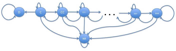
In this model, there are 2 absorbing states, D and NR. This means that every bond will eventually either default or stop being rated. This may be a case where the long-term predictions of a model which is chosen based on short-term dynamics, are unrealistic.
The estimated transition matrix for rating migrations over 1 year from one paper (which uses only AAA, AA, A, BBB, B, CCC, D and NR ratings) looks like this:
| NR | AAA | AA | A | BBB | BB | B | CCC | D | |
| NR | 0.9935 | 0.0000 | 0.0001 | 0.0003 | 0.0006 | 0.0009 | 0.0003 | 0.0000 | 0.0043 |
| AAA | 0.0248 | 0.8995 | 0.0640 | 0.0091 | 0.0005 | 0.0020 | 0.0001 | 0.0000 | 0.0001 |
| AA | 0.0321 | 0.0061 | 0.8788 | 0.0761 | 0.0057 | 0.0006 | 0.0004 | 0.0000 | 0.0001 |
| A | 0.0424 | 0.0004 | 0.0129 | 0.8944 | 0.0436 | 0.0047 | 0.0011 | 0.0002 | 0.0002 |
| BBB | 0.0545 | 0.0003 | 0.0023 | 0.0479 | 0.8479 | 0.0393 | 0.0063 | 0.0008 | 0.0008 |
| BB | 0.0965 | 0.0000 | 0.0012 | 0.0090 | 0.0869 | 0.7303 | 0.0612 | 0.0084 | 0.0065 |
| B | 0.1518 | 0.0001 | 0.0022 | 0.0024 | 0.0084 | 0.0643 | 0.6734 | 0.0534 | 0.0440 |
| CCC | 0.1429 | 0.0025 | 0.0003 | 0.0053 | 0.0017 | 0.0215 | 0.0674 | 0.3824 | 0.3760 |
| D | 0.0000 | 0.0000 | 0.0000 | 0.0000 | 0.0000 | 0.0000 | 0.0000 | 0.0000 | 1.0000 |
Note that, under this transition matrix, transitions from NR to other ratings can occur. Hence, the only absorbing state is D. Every bond eventually defaults.
If we are pessimistic and believe that every bond does eventually default, the probability that the bond goes into default or goes into non-rated is not the question in which the bond holder is most interested. Most bonds have a maturity and so the bond holder is interested in whether the bond will default before it matures. A more important calculation in this case is the probability of default before maturity. We will look at this question in subsequent weeks after going through and more carefully introducing Markov chains.
References
-
For details of mortgage default models, which are called roll rate models in the mortgage industry rather than Markov chains, see:
Davidson, Andrew and Levin, Alexander. Mortgage Valuation Models: Embedded Options, Risk, and Uncertainty, chapter 12. Oxford University Press, 2014.
-
For a reference to the matrix-theoretic approach to the calculation of absorption probabilities, see Theorem 3.3.9 of:
Kemeny, John G. and Snell, J. Laurie. Finite Markov Chains, chapter III. Springer, 1960.
This chapter focuses much more on calculating the absorption probabilities using a concept called the fundamental matrix which we do not pursue here.
-
Unfortunately, I know of no introductory reference to the graph-theoretic approach to the calculation of absorption probabilities. For an advanced reference, see:
Freidlin, Mark I. and Wentzell, Alexander D. Random Perturbations of Dynamical Systems, chapter 6. Springer, 3rd edition, 2012.
-
Here is a reference to one of many papers on applications of Markov chains to rating migration:
Lando, David and Skodeberg, Torben M. Analyzing rating transitions and rating drift with continuous observations. Journal of Banking and Finance 26 (2002), 423-444.