Algorithms
In this lecture, we will present dynamic programming which is used in valuing American-style derivatives as well as in calculating probabilities of hidden Markov models and optimal trading strategies as we will see later. Before presenting these specific applications, we first present dynamic programming in its more general algorithmic setting.
An algorithm is a precise specification for how to solve a certain problem. Problems can be things like:
- How to multiply two matrices
- How to find the communicating classes of a Markov chain
- How to find if there is a path between two vertices of a graph
- How to find if there is a path between two vertices of a graph which goes through every other vertex
- How to find the value of an American option on a binomial tree
Early on in the study of computer algorithms, people realized that the exact running time or number of operations is, in general, not a good measure of the performance of an algorithm. Over the years, hardware improves and so these measures change significantly. One way to better measure the performance is to look at how the number of operations grows with the size of the problem. In particular, it is common to look at the worst-case number of operations for any problem of a given size. Changes in hardware tend to make a program faster by a constant multiple, say twice as fast. However, the growth rate of the number of operations does not change.
Big $O$ Notation
We now discuss a commonly used measure of the growth rate of a function, which is invariant to constant multiples, called big $O$. A real function $f$ is big $O$ of $g$, written $f(x) = O\left(g(x)\right)$ with $g$ a real function if there is a positive real number $M$ and a real number $x_0$ such that: \begin{eqnarray} \left| f(x) \right| \leq M g(x) \end{eqnarray} for all $x > x_0$. $f(x) = O\left(g(x)\right)$ is roughly interpreted as $f(x)$ is smaller than or equal to $g(x)$, or, more precisely, $f(x)$ grows more slowly than or at the same rate as $g(x)$. The way this notation tends to be used in practice is that $g$ is chosen to be a simple function such as a monomial, an exponential or a logarithm. Big $O$ notation allows us to summarize the growth of $f$ in terms of the simpler functions $g$. Here are some examples and some simplification rules for big $O$:
- If $\lim_{x\rightarrow\infty} f(x) = \infty$ and $f(x) = O\left(g(x)\right)$ then, for any constant $c$, we have that $f(x) + c = O\left(g(x)\right)$
- If $f(x) = O\left(g(x)\right)$ then $c f(x) = O\left(g(x)\right)$
- If $f(x) = O\left(h(x)\right)$ and $g(x) = O\left(h(x)\right)$ then $f(x) + g(x) = O\left(h(x)\right)$
- For any integer $n$, we have that $x^n = O\left(x^{n+1}\right)$
- If $p(x)$ is an $n$th-order polynomial, then $p(x) = O\left(x^n\right)$
- If $p(x)$ is a polynomial, then $p(x) = O\left(\exp(x)\right)$
Example: Matrix Multiplication
We now present, as an example, the standard algorithm for matrix multiplication. The following code multiplies the matrix $M$ by the matrix $N$ and places the result in the matrix $P$:
      n = size(M,1)
      P = zeros( n, n )
      for i in 1:n
          for j in 1:n
              for k in 1:n
                  P[i,j] += M[i,k]*M[k,j]
              end
          end
      end
Notice that there are $3$ nested loops each of which performs $n$ iterations. Hence, the total number of operations is $O\left(n^3\right)$ where $n$ is the size of the matrix, that is, $M \in \mathbb{R}^{n\times n}$. The initial operations don't matter because this just adds a constant. We make a few additional comments on the matrix multiplication algorithm:
- The computational complexity of most algorithms is quoted in terms of the size of the input. For matrix multiplication, the size of the input is $O\left(n^2\right)$ since there are $n^2$ elements in a matrix. However, the academic literature usually quotes the running times of matrix algorithms as functions of $n$ rather than $n^2$.
- In fact, this is not the fastest known algorithm for the matrix multiplication problem. Strassen's algorithm performs matrix multiplication in $O\left(n^{2.81}\right)$. There is another known algorithm which runs in $O\left(n^{2.38}\right)$. However, these faster matrix multiplication algorithms are complex, have large hidden constants and are not numerically stable and so are not widely used. Note that any matrix multiplication algorithm has to look at every element of the matrices that it is multiplying and so must require at least $O\left(n^2\right)$.
- Matrix inversion, which might intuitively seem more complex than matrix multiplication, has the same performance as matrix multiplication ($O\left(n^3\right)$ using the standard algorithm and faster algorithms can be developed from faster matrix multiplication algorithms).
Communicating Classes of a Markov Chain
In this section, we explore the problem of finding the communicating classes of a Markov chain. As mentioned in previous lectures, this is a graph property, that is, it is dependent only on the graph of the Markov chain. Hence, we consider finding the communicating classes of a graph $G$.
For a graph $G$, recall that vertices $v$ and $v'$ communicate, written $v \leftrightarrow v'$ if there is a path from $v$ to $v'$ in the graph as well as a path from $v'$ to $v$. A set $C$ is a communicating class if and only if:
- For every $v, v'\in C$, we have $v\leftrightarrow v'$
- For every $v\in C$, if $v\leftrightarrow v'$ then $v'\in C$
	# vertices are labeled by positive integers
	# we label classes with the first vertex known to be in that class

	n = size(path,1)

	# list of all classes so far
	classes = Int[]

	# list of which class each vertex belongs to
	class = zeros( Int, n )

	for v1 = 1:n
	    for v2 in classes
	        if path[v1,v2] && path[v2,v1]
	            # v1 is in the class labeled v2
	            class[v1] = v2
	        end
	    end
    	    if class[v1] == 0
	        # v1 is in a new class
	        push!( classes, v1 )
	        class[v1] = v1
	    end
	end
We now analyze the complexity of this algorithm.
In the inner loop, the algorithm could, in the worst case, look at all classes which have been created up to that point.
When analyzing vertex $v1$ there are at most $v1-1$ classes, since every vertex could be in its own class.
Hence, the total number of operations is, in the worst case:
\begin{eqnarray}
\sum_{v=1}^n \left(v-1\right) = n\frac{n-1 + 0}{2} = O\left(n^2\right)
\end{eqnarray}
We now investigate how to find whether there is a path between vertex $v$ and $w$. We consider the brute force approach of enumerating all possible paths. Note that there are several ways of representing graphs in a computer and we pick one called an adjacency matrix. An adjacency matrix is a Boolean matrix, $\mbox{edge}$, such that $\mbox{edge}\left[v,v'\right]$ is $\mbox{true}$ if and only if there is an edge from vertex $v$ to vertex $v'$. Finding whether there is a path between the vertices of a graph can be easily implemented with recursion given the adjency matrix. For each vertex, we iterate through every other vertex, add it to the current path and then recursively calculate all paths starting from this:
          function findpaths!( edge, path = falses(size(edge,1),size(edge,1)), currpath = Int[] )
              for v in 1:size(edge,1)
                  if !( v in currpath )
                      if isempty(currpath) || edge[currpath[end], v]
                          push!( currpath, v )
                          path[currpath[1], v] = true
                          findpaths!( edge, path, currpath )
                          pop!( currpath )
                      end
                  end
              end
              return path
          end
Exponential versus Polynomial Time Algorithms
We now analyze the computational complexity of the above algorithm for finding which vertices are connected via directed paths in a directed graph.
The algorithm goes through each vertex which is not yet in the current path and which is connected to the current path at the end and recursively calls itself.
Let's assume that there are $n$ vertices and $m$ in the current path so far.
Let $T(n,m)$ denote the time the algorithm takes to calculate findapths! in this case.
If the graph is fully connected, there are $n-m$ vertices to go through and so:
\begin{eqnarray}
T(n,m) = (n-m)T(n,m+1)
\end{eqnarray}
with the end condition:
\begin{eqnarray}
T(n,n) = c
\end{eqnarray}
for some constant $c$.
Iterating the above formula, we see that:
\begin{eqnarray}
T(n,m) = (n-m)T(n,m+1) = (n-m)(n-m-1)T(n,m+2) = \ldots = (n-m)(n-m-1)\ldots 2 T(n,n) = (n-m)! c
\end{eqnarray}
The time to run the algorithm for an $n$ vertex fully connected graph starting with the empty path would be $T(n,0) = c n!$.
Note that $n!$ grows very rapidly, which can be seen from Stirling's formula:
\begin{eqnarray}
n! \sim \sqrt{2 \pi n} \left(\frac{n}{e}\right)^n
\end{eqnarray}
If $n\geq \alpha e$, we have:
\begin{eqnarray}
n! \sim \sqrt{2 \pi n} \left(\frac{n}{e}\right)^n \geq \sqrt{2 \pi n} \left(\frac{\alpha e}{e}\right)^n = \sqrt{2 \pi n} \left(\alpha\right)^n \geq \alpha^n
\end{eqnarray}
Hence, $\alpha^n = O\left(n!\right)$ for any $\alpha$.
The following chart shows how long the above program runs for up to $10$ vertices:
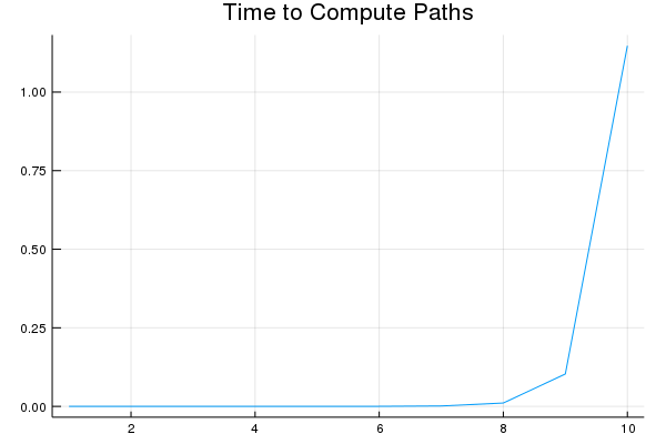
Notice that the amount of time is growing rapidly. In fact, if it is growing proportional to $n!$, then with the time per operation that this is taking, it will take many times the age of the universe to complete on $25$ vertices.
Note that while exponentials grow more slowly than the factorial, exponentials also grow fast. If the calculation were brought down to an exponential, say $2^n$, then it would take longer than the age of the universe to run with a Markov chain of $100$ vertices. We have talked about Markov chains that might involve 6,000 vertices and I've worked with Markov chains with 10's or 100's of thousands of vertices. On the other hand, using the dynamic programming algorithm we will talk about in the next section, we'll be able to achieve a computational complexity of $O\left(n^3\right)$ for the same problem and it will run on $100$ vertices in less than $0.004$ seconds. Computer scientists refer to problems which only have exponential time algorithms as intractable.
Dynamic Programming
The theory of algorithms involves a large number of stories. For almost every problem, and there are 10's of thousands of problems that computer scientists have investigated, there is a different approach required. There are very few general approaches which can be used to attack many different problems. However, dynamic programming is one of the few straightforward approaches that allows one to solve many algorithmic problems.
In our previous approach to finding if there is a path between each pair of vertices of a graph, we repeated certain computations many times. For example, for the path $3, 4, 5, 6$ is calculated in the process of calculating all of the following paths: \begin{eqnarray} 3, 4, 5, 6\\ 1, 3, 4, 5, 6\\ 1, 2, 3, 4, 5, 6\\ 1, 2, 7, 3, 4, 5, 6\\ \ldots\\ 2, 3, 4, 5, 6\\ 2, 1, 3, 4, 5, 6\\ 2, 1, 7, 3, 4, 5, 6\\ \ldots\\ \end{eqnarray} In total, this path is calculated 1,957 times. The idea behind dynamic programming is to avoid these repeated intermediate computations by storing some intermediate results.
Let's consider how we can calculate path without repeating intermediate computations. For a path $v_1, v_2, \ldots, v_k$, we call $v_1$ the starting point, $v_k$ the end point and other other vertices intermediate. Let's assume we've calculated all paths with intermediate vertices in the set $\left\{1,2,\ldots,m\right\}$ and we wish to calculate all paths with intermediate vertices $\left\{1,2,\ldots,m,m+1\right\}$. Here are the possibilities for such paths:
- The path only contains vertices from $\left\{1,2,\ldots,m\right\}$ in which case it has already been calculated.
- The path starts with vertex $m+1$ in which case it has already been calculated because all intermediate points are from $\left\{1,2,\ldots,m\right\}$.
- The path ends with vertex $m+1$ in which case it has already been calculated because all intermediate points are from $\left\{1,2,\ldots,m\right\}$.
- Vertex $m+1$ is intermediate in the path. This is the case which has not yet been calculated.
          function findpaths2!( edge )
              path = copy(edge)
              n = size(edge,1)
              for m = 1:n
                  path[m,m] = true
                  for v1 = 1:n
                      for vk = 1:n
                          if path[v1,m] && path[m,vk]
                              path[v1,vk] = true
                          end
                      end
                  end
              end
              return path
          end
The computational complexity of the above algorithm is easy to calculate. There are $3$ nested loops which each do $n$ iterations. Hence the complexity is $O\left(n^3\right)$. Note that this algorithm significantly extends the size of graphs that can be explored. For example, using this algorithm, we can solve the path problem for a graph with 10,000 vertices in less than an hour and a quarter whereas the previous algorithm takes over $7$ hours to solve the problem with 14 vertices.
Example: The Hamiltonian Path Problem
We mention a variant of the path problem which is believed to be intractable. Consider the problem of trying to determine if there is a path in a graph which contains all vertices of the graph. This is called the Hamitonian path problem. This problem is known to be in a class of problems which are called NP-complete. No polynomial time algorithm is known for any NP-complete problem. If there is a polynomial time algorithm for any one of these problems, then there is one for all of them. There are thousands of problems known to be in this class of problems. Most computer scientists believe that these problems are intractable. Notice that the Hamiltonian problem is a slight variant of the path problem that we demonstrated a polynomial time algorithm for. It often happens that not very different variants of tractable problems can be intractable. The question of whether there is a polynomial time algorithm for NP-complete problems is the most famous open problem in theoretical computer science.
The Application of Dynamic Programming to American Option Valuation
An option is a financial instrument which gives the owner the option of buying some asset at some fixed price $K$, referred to as the strike price. The option is American if it can be exercised at any time up to a maturity date $T$ and European if it can only be exercised on the maturity date. While European options are easy to evaluate, American options are more difficult and some of the popular methods to evaluate them are heuristic in nature. One very solid method for evaluating American options uses dynamic programming. We explore this in this section.
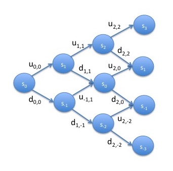
In order to value American options, we need to put a model on the underlying asset. Suppose the underlying asset behaves according to a Markov chain which can go up or down at each step such as this one. As an initial simplification, we assume that the self transitions have $0$ probability. We also relax the assumption of homogeneity so that the probability of going up, which we write as $u_{t,i}$, is dependent upon both the current time and the current value and similarly for the probability of going down, $d_{t,i}$. Note that in the finance literature, these non-homogeneous Markov chains are drawn differently than we have been drawing them. First, the states are drawn vertically rather than horizontally, that is, on top of each other rather than to the side. Second, since the Markov chains are non-homogeneous, the states are drawn for each time period with time going from left to right. Hence, the Markov chain looks like this:
We now consider valuing an American option on this model. We can value any contract as its future expected value under the assumption that the model is risk-neutral. Assuming $0$ interest rates, the model is risk-neutral if any any point, the value of the underlying asset is equal to its future expected value. We assume that the values of $u_{t,i}$ and $d_{t,i}$ have been chosen so that the model is risk-neutral.
Consider determining the future expected value of an option at time $0$. At this time, the owner can exercise the option, in which case the future expected value is its current value less the strike price $K$, or hold it, in which case we need to look at subsequent steps. At the next step, the market can go up or down. At each of these steps, the same decision must be made. Hence, using brute force, we would need to iterate through all possible paths that the Markov chain can take through the binomial tree. Since at each step, the process can either go up or down. That means that if there are $T$ steps until maturity, there will be a total of $2^T$ paths. Hence, this brute force approach would be exponential in the number of steps.
In the above discussion, we evaluate the American option on each state of the Markov chain multiple times. For example, one path goes up and then down and leaves us in state $s_0$. Another path goes down and then up but also leaves us in state $s_0$. Since all information about the future evolution of the process is contained in the current state of a Markov chain, we need only evaluate each state once. Let $v_{t,i}$ denote the value of the American option (with strike $K$ and maturity $T$) at time $t$ and state $s_i$. We equate the state $s_i$ with the value of the underlyer so the value of the option at time $t-1$ and in state $s_i$ is given by: \begin{eqnarray} v_{t-1,i} = \max\left(s_i - K, u_{t-1,i} v_{t,i+1} + d_{t-1,i} v_{t,i-1}\right)\\ \end{eqnarray} At maturity, if the owner doesn't sell the option, the value is $0$ so that the value of the option is given by: \begin{eqnarray} v_{T,i} = \max\left(s_i - K, 0\right) \end{eqnarray} With these formulas, we only need to evaluate the American option at each state. Hence, the total number of evaluations is given by the number of states which is: \begin{eqnarray} \sum_{t=0}^T \left(t+1\right) = (T+1)\frac{1 + T + 1}{2} = \frac{T \left(T + 2\right)}{2} \end{eqnarray} which is $O\left(T^2\right)$.
We finish with a few comments about dynamic programming for American option evaluation.
- To evaluate each state, we need to know the values of states which that state can reach in the future. Hence, we need to go backwards in time which is sometimes referred to as backward induction.
- Notice that a major assumption required for this approach to work is that the process is Markovian. Hence, it works for, for example, trinomial trees where the self transitions have non-zero probability.
- In addition to the Markov property, in order for this approach to be tractable, the process must not have an exponential number of states in the number of steps. If for example, the process goes up and down by different amounts each time step in such a way that the paths don't come together (e.g. up and down ends up as a different state than down and up), then there will be one state for every path at each time period. This type of tree has an exponential number of states as a function of time step and is referred to as non-recombining.
- This approach can be used for derivatives other than options. However, if the exercise value of the derivative is dependent upon the entire path, this approach will not work. Such derivatives are referred to as path dependent. As an example of a path-dependent option, Asian options are options which depend on the average price over time of the underlying asset.
- In some cases, options are dependent upon a number of different assets. If, for example, an option is dependent upon $2$ assets, one could build a Markov chain on the pair $\left(s_i,s_j'\right)$ of values of the different assets. While the number of states at time $t$ for a single asset option is $t$, for $2$ asset options, it will be $t^2$ (the product of the number of possible values of each asset). In this case, the running time of dynamic programming will be $O\left(T^3\right)$. In general, for $k$ asset options, the running time will be $O\left(T^{k+1}\right)$. Notice that this is exponential in the number of assets and can become intractable for large numbers of assets. This is important, for example, in mortgage bonds and CDO's, deals that are based on hundreds or thousands of underlying assets and that have complicated structure on top of them.
References
-
For material on algorithms, see the following chapters of the subsequent book:
- For a general introduction to algorithms, see chapter 1.
- For big O notation, see chapter 2.
- For dynamic programming, see chapter 16.
Cormen, Thomas H., Leiserson, Charles E. and Rivest, Ronald L. Introduction to Algorithms. MIT Press, 1985.
-
For material on the valuation of American options using binomial trees, see the following book. Note this book doesn't refer to this as dynamic programming but, from the perspective of computer science, that is the correct term.
Shreve, Steven E. Stochastic Calculus for Finance I, chapter 4. Springer, 2004.