Hidden Markov Models
We now introduce a class of models called hidden Markov models (HMM's), or, in much of the finance literature, regime-switching models. These models have an underlying state whose behavior is controlled by a Markov chain. However, the states of this Markov chain are not directly observable. Observable outcomes are drawn according to a probability distribution associated with each state. An example of this type of behavior is the $2$ state regime-switching model. This model can be viewed as a model of asset bubbles and financial crises: when the market is in the asset bubble, the market goes up with relatively low vol and when the market is in a financial crisis, the market goes down at a faster average rate but with higher volatility. Markets tend to be driven by panic and hype. We don't get to directly observe this behavior: we don't know how many investors in the market are excited about a given stock and so buying it and how many are afraid for its future and so selling it. We can mostly observe this behavior through its effect on the markets. Also, these models allow us to transform discrete Markov chains into continuous random variables, which many consider to more accurately model market prices.
To set up notation, let $s_1, s_2, \ldots, s_m$ be the states of the Markov chain. Let $\pi_0$ be its initial probability vector and $P$ the transition probabilities. Note that while the underlying Markov chain is discrete, we allow the observables of the hidden Markov model to be continuous random variables. Let $x_1, x_2, \ldots, x_n$ the sequence of states visited by the hidden Markov chain random variables $X_1, X_2, \ldots, X_n$. We assume that the observable random variables $Y_1, Y_2, \ldots, Y_n$ are such that $Y_i$ is conditionally independent of all other random variables given $X_i$ with density $f\left(Y_i|X_i\right)$. Let $y_1, y_2, \ldots, y_n$ be the sequence of observations of $Y_1, Y_2, \ldots, Y_n$. The probability (or, more accurately, probability density) of the observations and states is given by: \begin{eqnarray*} f_\theta{\left(x^n,y^n\right)} = \pi_{x_1} \prod_{i=2}^n P_{x_{i-1},x_i} \prod_{i=1}^n f\left(\left.y_i\right|x_i\right) \end{eqnarray*} where $\theta$ is a vector of parameters that include the initial and transition probabilities of the hidden Markov chain, and any parameters of the density of the observations in each state. We refer to this as the joint likelihood function. Since we don't observe $x_1, x_2, \ldots, x_n$, we are interested in the marginal probability of the observations $y_1, \ldots, y_n$ which is given by: \begin{eqnarray} f_\theta{\left(y^n\right)} = \sum_{x_1, x_2, \ldots, x_n} f_\theta{\left(x^n,y^n\right)} = \sum_{x_1, x_2, \ldots, x_n}\pi_{x_1} \prod_{i=2}^n P_{x_{i-1},x_i} \prod_{i=1}^n f\left(\left.y_i\right|x_i\right)\label{eq:likelihood} \end{eqnarray} This is the likelihood function. Note that the number of possible values for $x_i$ is $m$ so the number of total values for $x_1, x_2, \ldots, x_n$ is $m^n$. This grows very fast: if $n=100$ and $m=3$, this is more than $10^{47}$, which is not feasible on any computer which is likely to be available any time soon. The computation time is $O\left(m^n\right)$. Hence, it is rarely possible to evaluate (\ref{eq:likelihood}) directly. We now look at ways of calculating this quantity efficiently through dynamic programming.
First we define the forward probabilities: \begin{eqnarray*} \alpha_t(i) = f_\theta{\left(y^t, x_t=s_i\right)} \end{eqnarray*} where $y^t$ denotes the first $t$ observations, $y_1, y_2, \ldots, y_t$. Note that, if we can efficiently calculate $\alpha_n(i)$, we can calculate the likelihood as: \begin{eqnarray*} f_\theta{\left(y^n\right)} = \sum_{i=1}^m f_\theta{\left(y^n, x_n=s_i\right)} = \sum_{i=1}^m\alpha_n(i) \end{eqnarray*} In fact, there is a dynamic programming approach to calculate $\alpha_t(i)$: \begin{eqnarray*} \alpha_{t+1}(i) & = & f_\theta{\left(y^{t+1}, x_{t+1}=s_i\right)} = \sum_{j=1}^m f_\theta{\left(y^{t+1}, x_t=s_j, x_{t+1}=s_i\right)} = \sum_{j=1}^m f_\theta{\left(y^t, x_t=s_j, x_{t+1}=s_i\right)} f{\left(\left.y_{t+1}\right|x_{t+1}=s_i\right)}\\ & = & \sum_{j=1}^m f_\theta{\left(y^t, x_t=s_j\right)} P_{s_j,s_i} f\left(\left.y_{t+1}\right|x_{t+1}=s_i\right) = \sum_{j=1}^m \alpha_t(j) P_{s_j,s_i} f\left(\left.y_{t+1}\right|x_{t+1}=s_i\right) \end{eqnarray*} Using the initial condition $\alpha_1(i) = \pi_i f_{s_i}{\left(y_1\right)}$, this enables us to calculate the likelihood function in $O\left(n\times m^2\right)$, which is dramatically better than $O\left(n m^n\right)$ from directly calculating the likelihood. For example, for the previous example of $n=100$ and $m=3$, this calculation requires around $900$ steps where the direct calculation requires more than $10^{49}$.
Local Maxima
We now have the ability to calculate the likelihood of the hidden Markov models. We would like to fit such models. Previously, we discussed maximum likelihood estimation. In the examples that we gave, we were able to solve for an explicit formula for the maximum likelihood estimator of several different models. In the case of hidden Markov models, there is no known formula for the maximum likelihood estimator.
If a maximization problem is strictly concave, then there is a unique maximum. For all the problems that we explored in the lecture on fitting models, the log likelihood function was concave in the parameters. However, in practice, the log likelihood function (or many other objectives that are commonly used) for many problems is not concave, making maximization much more difficult. For hidden Markov models, the log likelihood function is not concave. In fact, the HMM log likelihood function often has many local maxima.
Consider a hidden Markov model with an underlying Markov chain having all possible edges, referred to as fully connected:
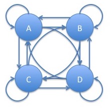
In this case, if we were to relabel $A$ to $B$ and vice versa in the graph and transition matrix, we get the exact same distribution of the observable process. In particular, let $\sigma$ be the permutation of $A$ and $B$, that is: \begin{eqnarray*} \sigma\left(s\right) = \left\{\begin{array}{rl} B & \mbox{if $s=A$}\\ A & \mbox{if $s=B$}\\ s & \mbox{if $s\ne A$ and $s\ne B$}\\ \end{array}\right. \end{eqnarray*} We then transform the transition and initial probabilities and densities from $\pi$, $p$ and $f$ into $\pi'$, $p'$ and $f'$: \begin{eqnarray*} \pi'_s & = & \pi_{\sigma(s)}\\ p'_{s,t} & = & p_{\sigma(s),\sigma(t)}\\ f'\left(\left.y\right| x=s\right) & = & f_{\sigma(s)}(y)\\ \end{eqnarray*} Then, the distribution of the observable random variables, $Y_1, Y_2, \ldots$ will be exactly the same as the original hidden Markov model: \begin{eqnarray*} f'_{\theta'}{\left(y^n\right)} & = & \sum_{x_1, x_2, \ldots, x_n} f'_{\theta'}{\left(x^n,y^n\right)} = \sum_{x_1, x_2, \ldots, x_n}\pi'_{x_1} \prod_{i=2}^n P'_{x_{i-1},x_i} \prod_{i=1}^m f'\left(\left.y_i\right|x_i\right)\\ & = & \sum_{x_1, x_2, \ldots, x_n}\pi_{\sigma{\left(x_1\right)}} \prod_{i=2}^n P_{\sigma{\left(x_{i-1}\right)},\sigma{\left(x_i\right)}} \prod_{i=1}^m f_{}{\left(\left.y_i\right|\sigma{\left(x_i\right)}\right)}\\ & = & \sum_{x'_1, x'_2, \ldots, x'_n}\pi_{x'_1} \prod_{i=2}^n P_{x'_{i-1},x'_i} \prod_{i=1}^m f{\left(\left.y_i\right|x'_i\right)} = f_\theta{\left(y^n\right)}\\ \end{eqnarray*}
Note that the same result will hold for any permutation of the labels of the graph of the Markov chain and corresponding parameters. There are $m!$ such permutations so this means, that if there is some local maximum $\hat{\theta}$ of the log likelihood function, there will be $m!$ such local maxima obtained by permuting the labels of the states and corresponding parameters. As previously discussed, $m!$ grows very fast, in fact, faster than any exponential. For $m=5$, this yields $120$ local maxima and for $m=10$, it yields $3,628,800$. Also, these may not be the only local maxima that occur.
Expectation Maximization
In this section, we discuss an iterative technique for finding local maxima of the log likelihood function called expectation maximization or EM. The EM algorithm iteratively performs the following maximization: \begin{eqnarray}\label{EM} \theta^{k+1} = \mbox{arg max}_\theta E_{\theta^k}{\left[\log f_\theta{\left(X^n, Y^n\right)}\right|\left.Y^n\right]} \end{eqnarray} First a few remarks about the right hand side of (\ref{EM}):
- There are two occurences of parameter vectors, $\theta$ in (\ref{EM}): one in the joint likelihood function and one in the expectation. The optimization is over the parameter vector in the joint likelihood function.
- The expectation is conditional on the observations $Y^n$. Hence, the criterion we are maximizing can be viewed as the expected value of the log likelihood of the hidden states given the observations.
It turns out that this procedure always increases the log likelihood function unless we are at a local maximum. In order to demonstrate this, we first repeat Jensen's inequality in a fuller version:
For any convex function $f:\mathbb{R}\rightarrow\mathbb{R}$ and any random variable $X$: \begin{eqnarray*} E{\left[f{\left(X\right)}\right]}\geq f{\left(E{\left[X\right]}\right)} \end{eqnarray*} Furthermore, if $f$ is strictly convex, then equality holds in the above if and only if $X$ is a constant.
We can now show that the sequence of estimates generated by the EM algorithm will monotonically increase:
Let $\theta^k$ be a sequence of parameter estimates a a hidden Markov model determined according to (\ref{EM}), then: \begin{eqnarray*} f_{\theta^{k+1}}{\left(y^n\right)} \geq f_{\theta^k}{\left(y^n\right)} \end{eqnarray*}
We first summarize the proof into the following steps:
- In place of (\ref{EM}), we can choose: \begin{eqnarray*} \mbox{arg max}_\theta E_{\theta^k}{\left[\left.\log {\left(\frac{f_\theta{\left(X^n, Y^n\right)}}{f_{\theta^k}{\left(X^n\right|\left.Y^n\right)}}\right)}\right|Y^n\right]} \end{eqnarray*} which, while computationally less attractive, will facilitate the proof.
- We have that: \begin{eqnarray*} E_{\theta^k}{\left[\left.\log\left(\frac{f_\theta{\left(X^n,Y^n\right)}}{f_{\theta^k}{\left(X^n\right|\left.Y^n\right)}}\right)\right|Y^n=y^n\right]} \leq \log f_\theta{\left(y^n\right)} \end{eqnarray*}
- Equality holds in the above, that is: \begin{eqnarray*} E_{\theta^k}{\left[\left.\log\left(\frac{f_{\theta^k}{\left(X^n,Y^n\right)}}{f_{\theta^k}{\left(X^n\right|\left.Y^n\right)}}\right)\right|Y^n=y^n\right]} = \log f_{\theta^k}{\left(y^n\right)} \end{eqnarray*} if and only if $\theta=\theta^k$.
- Putting all this together yields: \begin{eqnarray*} \log \left(f_{\theta^k}{\left(y^n\right)}\right) & = & E_{\theta^k}{\left[\left.\log\left(\frac{f_{\theta^k}{\left(X^n,Y^n\right)}}{f_{\theta^k}{\left(X^n\right|\left.Y^n\right)}}\right)\right|Y^n=y^n\right]}\\ & \leq & \max_\theta E_{\theta^k}{\left[\left.\log\left(\frac{f_\theta{\left(X^n,Y^n\right)}}{f_{\theta^k}{\left(X^n\right|\left. Y^n\right)}}\right)\right|Y^n=y^n\right]}\\ & = & E_{\theta^k}{\left[\left.\log\left(\frac{f_{\theta^{k+1}}{\left(X^n,Y^n\right)}}{f_{\theta^k}{\left(X^n\right|\left.Y^n\right)}}\right)\right|Y^n=y^n\right]}\\ & \leq & \log\left(f_{\theta^{k+1}}{\left(y^n\right)}\right) \end{eqnarray*}
- To see this, notice that: \begin{eqnarray*} \lefteqn{\mbox{arg max}_\theta E_{\theta^k}{\left[\log f_\theta{\left(X^n, Y^n\right)}\right|\left.Y^n\right]}}\\ & = & \mbox{arg max}_\theta E_{\theta^k}{\left[\left.\log f_\theta{\left(X^n, Y^n\right)}\right|Y^n\right]} - E_{\theta^k}{\left[\left.\log f_{\theta^k}{\left(X^n\right|\left.Y^n\right)}\right|Y^n\right]}\\ & = & \mbox{arg max}_\theta E_{\theta^k}{\left[\left.\log {\left(\frac{f_\theta{\left(X^n, Y^n\right)}}{f_{\theta^k}{\left(X^n\right|\left.Y^n\right)}}\right)}\right|Y^n\right]} \end{eqnarray*}
- Since $\log$ is a concave function, Jensen's inequality implies: \begin{eqnarray*} \lefteqn{E_{\theta^k}{\left[\left.\log\left(\frac{f_\theta{\left(X^n,Y^n\right)}}{f_{\theta^k}{\left(X^n\right|\left.Y^n\right)}}\right)\right|Y^n=y^n\right]}}\\ & \leq & \log \left(E_{\theta^k}{\left[\left.\frac{f_\theta{\left(X^n,Y^n\right)}}{f_{\theta^k}{\left(X^n\right|\left.Y^n\right)}}\right|Y^n=y^n\right]}\right) = \log \left(\sum_{x^n} \frac{f_\theta{\left(x^n,y^n\right)}}{f_{\theta^k}{\left(x^n\right|\left.y^n\right)}} f_{\theta^k}{\left(x^n\right|\left.y^n\right)}\right) = \log \left(\sum_{x^n} f_\theta{\left(x^n,y^n\right)}\right) = \log f_\theta{\left(y^n\right)} \end{eqnarray*}
- Jensen's inequality tells us that we have equality if and only if: \begin{eqnarray*} \frac{f_\theta{\left(x^n,y^n\right)}}{f_{\theta^k}{\left(x^n\right|\left.y^n\right)}} = c \end{eqnarray*} for all $x^n$ and some constant $c$. Here, $c$ can be dependent upon $y^n$ since we are assuming $y^n$ is fixed. The above holds when $\theta=\theta^k$ since: \begin{eqnarray*} \frac{f_{\theta^k}{\left(x^n,y^n\right)}}{f_{\theta^k}{\left(x^n\right|\left.y^n\right)}} = \frac{f_{\theta^k}{\left(x^n\right|\left.y^n\right)}f_{\theta^k}{\left(y^n\right)}}{f_{\theta^k}{\left(x^n\right|\left.y^n\right)}} = f_{\theta^k}{\left(y^n\right)} \end{eqnarray*}
Note that the fact that the objective is nondecreasing does not necessarily imply that the iterative technique will converge or, if it converges, that it will converge to a local maximum:
- For example, for the sequence $x_n = (-1)^n\left(1+2^{-n}\right)$, the function $f(x) = -x^2$ is always increasing, that is, $f\left(x_n\right) < f\left(x_{n+1}\right)$ for every $n$. However, this sequence oscillates and so does not converge.
- For the sequence $x_n = 1+2^{-n}$, the function $f(x) = -x^2$ is always increasing, that is, $f\left(x_n\right) < f\left(x_{n+1}\right)$ for every $n$. However, this sequence converges to $1$ whereas the only local maximum of the function is at $0$.
Under conditions, the EM algorithm converges to a local maximum.
Expectation-Maximization for HMM's
We now specialize (\ref{EM}) to HMM's. We need to maximize over $\theta$: \begin{eqnarray} E_{\theta^k}{\left[\log f_\theta{\left(X^n, Y^n\right)}\right|\left.Y^n=y^n\right]} & = & E_{\theta^k}{\left[\left.\log \left(\pi_{X_1} \prod_{i=2}^n P_{X_{i-1},X_i} \prod_{i=1}^m f\left(\left.Y_i\right|X_i\right)\right)\right|Y^n=y^n\right]}\nonumber\\ & = & E_{\theta^k}{\left[\left.\log \pi_{X_1} + \sum_{i=2}^n \log P_{X_{i-1},X_i} + \sum_{i=1}^n \log f\left(\left.Y_i\right|X_i\right)\right|Y^n=y^n\right]}\nonumber\\ & = & E_{\theta^k}{\left[\left.\log \pi_{X_1}\right|Y^n=y^n\right]} + E_{\theta^k}{\left[\left.\sum_{i=2}^n\sum_{j=1}^m\sum_{j'=1}^m n_{s_j,s_{j'}}{\left(X_{i-1}X_i\right)}\log P_{s_j,s_{j'}}\right|Y^n=y^n\right]} + E_{\theta^k}{\left[\left.\sum_{i=1}^n \sum_{j=1}^m n_{s_j}{\left(X_i\right)}\log f\left(\left.Y_i\right|x_i=s_j\right)\right|Y^n=y^n\right]}\label{Q}\\ \end{eqnarray} subject to the constraints $\sum_{j'=1}^m P_{s_j,s_{j'}} = 1$. We will add each of these constraints using the Lagrange multiplier $\lambda_j$. We will solve for the transition probabilities and for the parameters of the observation distribution separately. We assume the initial distribution is known.
EM for the transition probabilities
We first maximize over $P_{s_j,s_{j'}}$ by setting the derivative equal to $0$: \begin{eqnarray*} \lefteqn{\frac{\partial}{\partial P_{s_j,s_{j'}}} \left(E_{\theta^k}{\left[\log f_\theta{\left(X^n, Y^n\right)}\right|\left.Y^n=y^n\right]} + \sum_{j=1}^m \lambda_j \sum_{j'=1}^m P_{s_j,s_{j'}}\right)}\\ & = & \frac{\partial}{\partial P_{s_j,s_{j'}}} \left(E_{\theta^k}{\left[\left.\sum_{i=2}^n\sum_{j=1}^m\sum_{j'=1}^m n_{s_j,s_{j'}}{\left(X_{i-1}X_i\right)}\log P_{s_j,s_{j'}}\right|Y^n=y^n\right]} + \sum_{j=1}^m \lambda_j \sum_{j'=1}^m P_{s_j,s_{j'}}\right)\\ & = & E_{\theta^k}{\left[\left.\sum_{i=2}^n\frac{n_{s_j,s_{j'}}{\left(X_{i-1}X_i\right)}}{P_{s_j,s_{j'}}}\right|Y^n=y^n\right]} + \lambda_j = 0\\ \end{eqnarray*} Hence: \begin{eqnarray*} P_{s_j,s_{j'}} & = & -\sum_{i=2}^nE_{\theta^k}{\left[\left.\frac{n_{s_j,s_{j'}}{\left(X_{i-1}X_i\right)}}{\lambda_j}\right|Y^n=y^n\right]} \end{eqnarray*} Solving for $\lambda_i$ using the constraint yields: \begin{eqnarray*} \sum_{j'=1}^m P_{s_j,s_{j'}} = -\sum_{j'=1}^m \sum_{i=2}^nE_{\theta^k}{\left[\left.\frac{n_{s_j,s_{j'}}{\left(X_{i-1}X_i\right)}}{\lambda_j}\right|Y^n=y^n\right]} = 1 \end{eqnarray*} which means: \begin{eqnarray*} \lambda_j = -\sum_{j'=1}^m \sum_{i=2}^nE_{\theta^k}{\left[\left.n_{s_j,s_{j'}}{\left(X_{i-1}X_i\right)}\right|Y^n=y^n\right]} \end{eqnarray*} so that: \begin{eqnarray*} P^{k+1}_{s_j,s_{j'}} & = & \frac{\sum_{i=2}^nE_{\theta^k}{\left[\left.n_{s_j,s_{j'}}{\left(X_{i-1}X_i\right)}\right|Y^n=y^n\right]}}{\sum_{j'=1}^m \sum_{i=2}^nE_{\theta^k}{\left[\left.n_{s_j,s_{j'}}{\left(X_{i-1}X_i\right)}\right|Y^n=y^n\right]}} \end{eqnarray*} where $P^{k+1}$ denotes the transition probabilities of $\theta^{k+1}$, the parameters corresponding to the next iteration. In order to calculate this, we use: \begin{eqnarray*} \lefteqn{E_{\theta^k}{\left[\left.n_{s_j,s_{j'}}{\left(X_{i-1}X_i\right)}\right|Y^n=y^n\right]}}\\ & = & \mathbb{P}\left(\left.X_{i-1}=s_j, X_i=s_{j'}\right|Y^n=y^n\right)\\ & = & f_{\theta^k}{\left(\left.x_{i-1}=s_j,x_i=s_{j'}\right|y^n\right)}\\ & = & \frac{f_{\theta^k}{\left(x_{i-1}=s_j,y^{i-1}\right)}P^k_{s_j,s_{j'}}f\left(\left.y_i\right|x_i=s_{j'}\right)f_{\theta^k}{\left(\left.y^{>i}\right|x_i=s_{j'}\right)}}{f_{\theta_k}{\left(y^n\right)}} \end{eqnarray*} where $y^{>i} = y_{i+1} y_{i+2} \ldots y_n$. Note that the first factor in the numerator of the last expression is one of the forward probabilities. The last factor in this expression is called the backward probability and is denoted by $\beta_i(j)$. The backward probabilities can be calculated in a similar way to the forward probabilities: \begin{eqnarray*} \beta_i(j) & = & f_{\theta^k}{\left(\left.y^{>i}\right|x_i=s_{j'}\right)}\\ & = & \sum_{j''=1}^m f\left(\left.y_{i+1}\right|x_{i+1}=s_{j''}\right)P^k_{s_{j'},s_{j''}}f_{\theta^k}{\left(\left.y^{>i+1}\right|x_{i+1}=s_{j''}\right)}\\ & = & \sum_{j''=1}^m f\left(\left.y_{i+1}\right|x_{i+1}=s_{j''}\right)P^k_{s_{j'},s_{j''}}\beta_{i+1}{\left(j''\right)} \end{eqnarray*} Putting all this together we get: \begin{eqnarray*} P^{k+1}_{s_j,s_{j'}} = \frac{\sum_{i=2}^n \alpha_j(i-1) P^k_{s_j,s_{j'}} f_{s_{j'}}{\left(y_i\right)}\beta_{j'}(i)}{\sum_{j'=1}^m\sum_{i=2}^n \alpha_j(i-1) P^k_{s_j,s_{j'}} f_{s_{j'}}{\left(y_i\right)}\beta_{j'}(i)} \end{eqnarray*} and there are recursive formulas for $\alpha_j(i-1)$ and $\beta_{j'}(i)$.
EM for the parameters of the distribution of observations
We will now optimize for the parameters of the distribution of observations, $f_s\left(y_i\right)$. There are many ways of parameterizing distributions so we focus on the particular distribution which will interest us in this lecture, that is, the lognormal distribution. Given that the process is in state $s_j$, we will assume that the output distribution is lognormal with parameters $\mu_j$ and $\sigma_j$. We will write $f_{\mu_j,\sigma_j}$ in place of $f_{s_j}$ as we had been writing. Note that, if $Y_i$ is log normally distributed, then $\log Y_i$ is normally distributed and we will use the normal distribution to make the calculations slightly easier. We now set the derivatives of (\ref{Q}) with respect to $\mu_j$ to $0$: \begin{eqnarray*} \lefteqn{\frac{\partial}{\partial \mu_j} \left(E_{\theta^k}{\left[\log f_\theta{\left(X^n, Y^n\right)}\right|\left.Y^n=y^n\right]} + \sum_{j=1}^m \lambda_j \sum_{j'=1}^m P_{s_j,s_{j'}}\right)}\\ & = & \frac{\partial}{\partial \mu_j}\left(E_{\theta^k}{\left[\left.\log \pi_{X_1}\right|Y^n=y^n\right]} + E_{\theta^k}{\left[\left.\sum_{i=2}^n\sum_{j=1}^m\sum_{j'=1}^m n_{s_j,s_{j'}}{\left(X_{i-1}X_i\right)}\log P_{s_j,s_{j'}}\right|Y^n=y^n\right]} + E_{\theta^k}{\left[\left.\sum_{i=1}^n \sum_{j=1}^m n_{s_j}{\left(X_i\right)} \log f{\left(\left.Y_i\right|x_i=s_j\right)}\right|Y^n=y^n\right]}\right)\\ & = & \frac{\partial}{\partial \mu_j}E_{\theta^k}{\left[\left.\sum_{i=1}^n \sum_{j=1}^m n_{s_j}{\left(X_i\right)}\log f_{\mu_j,\sigma_j}{\left(Y_i\right)}\right|Y^n=y^n\right]}\\ & = & \frac{\partial}{\partial \mu_j}E_{\theta^k}{\left[\left.\sum_{i=1}^n n_{s_j}{\left(X_i\right)}\left(\frac{1}{2}\log\left(2\pi\sigma_j^2\right) - \frac{\left(\log\left(Y_i\right) - \mu_j\right)^2}{2\sigma_j^2}\right)\right|Y^n=y^n\right]}\\ & = & \sum_{i=1}^n E_{\theta^k}{\left[\left.n_{s_j}{\left(X_i\right)} \frac{\log\left(Y_i\right) - \mu_j}{\sigma_j^2}\right|Y^n=y^n\right]} = 0\\ \end{eqnarray*} Hence: \begin{eqnarray*} \mu_j = \frac{\sum_{i=1}^n \log\left(y_i\right)E_{\theta^k}{\left[\left.n_{s_j}{\left(X_i\right)}\right|Y^n=y^n\right]}}{\sum_{i=1}^n E_{\theta^k}{\left[\left.n_{s_j}{\left(X_i\right)}\right|Y^n=y^n\right]}} \end{eqnarray*} In order to calculate this, we use: \begin{eqnarray*} \lefteqn{E_{\theta^k}{\left[\left.n_{s_j}{\left(X_i\right)}\right|Y^n=y^n\right]}}\\ & = & \mathbb{P}\left(\left.X_i=s_j\right|Y^n=y^n\right)\\ & = & \frac{f_{\theta^k}{\left(x_i=s_j,y^i\right)} f_{\theta^k}{\left(\left.y^{>i}\right|x_i=s_j\right)}}{f_{\theta^k}{\left(y^n\right)}}\\ & = & \frac{\alpha_i(j)\beta_i(j)}{\sum_{j=1}^m\alpha_n(j)} \end{eqnarray*} Putting this algother yields: \begin{eqnarray*} \mu^{k+1}_j = \frac{\sum_{i=1}^n \log\left(y_i\right) \alpha_i(j)\beta_i(j)}{\sum_{i=1}^n\alpha_i(j)\beta_i(j)} \end{eqnarray*} By a similar argument, it can be shown that: \begin{eqnarray*} \sigma^{k+1}_j = \sqrt{\frac{\sum_{i=1}^n \left(\log\left(y_i\right) - \mu^{k+1}_j\right)^2 \alpha_i(j)\beta_i(j)}{\sum_{i=1}^n\alpha_i(j)\beta_i(j)}} \end{eqnarray*}
Summary
We now summarize the the EM algorithm for HMM's:- Initialization:
- Initialize $P^0$ to be an arbitrary $m\times m$ transition matrix
- Initialize $\mu^0$ to be an arbitrary $m$-vector
- Initialize $\sigma^0$ to be an arbitrary positive $m$-vector
-
Perform the following iteration for each $k$ until an appropriate termination condition is met:
-
Calculate the forward probabilities:
- Intialization: for $i$ from $1$ to $m$: \begin{eqnarray*} \alpha_0(i) = \pi_{s_i} \end{eqnarray*}
- For $t$ from $1$ to $n$ and $i$ from $1$ to $m$: \begin{eqnarray*} \alpha_{t+1}(i) = \sum_{j=1}^m \alpha_t(j) P^k_{s_j,s_i} f_{\mu^k_i,\sigma^k_i}{\left(y_{t+1}\right)} \end{eqnarray*}
-
Calculate the backward probabilities:
- Initialization: for $i$ from $1$ to $m$: \begin{eqnarray*} \beta_n(i) = 1 \end{eqnarray*}
- For $t$ from $n-1$ to $1$ and $i$ from $1$ to $m$: \begin{eqnarray*} \beta_t(i) = \sum_{j=1}^m \beta_{t+1}{\left(j\right)}P^k_{s_i,s_j}f_{\mu^k_j,\sigma^k_j}{\left(y_{t+1}\right)} \end{eqnarray*}
- Calculate $P^{k+1}$: for $i$ from $1$ to $m$ and $j$ from $1$ to $m$ \begin{eqnarray*} P^{k+1}_{s_i,s_j} = \frac{\sum_{t=2}^n \alpha_i(t-1) P^k_{s_i,s_j} f_{\mu_j,\sigma_j}{\left(y_t\right)}\beta_j(t)}{\sum_{j=1}^m\sum_{t=2}^n \alpha_i(t-1) P^k_{s_i,s_j} f_{s_j}{\left(y_t\right)}\beta_j(t)} \end{eqnarray*}
- Calculate $\mu^{k+1}$: for $i$ from $1$ to $m$: \begin{eqnarray*} \mu^{k+1}_i = \frac{\sum_{t=1}^n \log\left(y_t\right) \alpha_t(i)\beta_t(i)}{\sum_{t=1}^n\alpha_t(i)\beta_t(i)} \end{eqnarray*}
- Calculate $\sigma^{k+1}$: for $i$ from $1$ to $m$: \begin{eqnarray*} \sigma^{k+1}_i = \sqrt{\frac{\sum_{t=1}^n \left(\log\left(y_t\right) - \mu^{k+1}_i\right)^2 \alpha_t(i)\beta_t(i)}{\sum_{t=1}^n\alpha_t(i)\beta_t(i)}} \end{eqnarray*}
-
Calculate the forward probabilities:
Practicalities of Fitting HMM's
Scaling
Note that the calculations of the forward and backward probabilities involve products of numbers across each observation. Since there are often hundreds or thousands of observations, this can easily lead to overflow or underflow. One way to deal with this is to keep track of a scaling factor for the sum of the forward or backward probabilities at each step. Notice that all of the update equations are invariant to a scaling factor on the forward or backward probabilities. Hence, we can scale these probabilities so that they sum to $1$ at each step. Note that, if one wishes to calculate the likelihood, the intermediate scale factors must be kept track of.
Termination condition
There are several possible rules one might use to terminate the iterations of the EM algorithm. One could stop when $\theta^k$ and $\theta^{k+1}$ are sufficiently close, for example. However, since it is the likelihood that we are ultimately trying to optimize, I prefer to stop when the likelihood between two iterations improves by less than a certain percentage. In particular, the termination condition used in the experiments below is when the likelihood changes by less than $0.01$bp.
Local maxima
As mentioned previously, the likelihood of hidden Markov models may have many local maxima. There is no known approach to guarantee that one finds the global maximum. One approach for dealing with this is to run with multiple random starting parameter sets and choose the parameter set which has the highest likelihood. This is the approach that I take: I run the EM algorithm $200$ times with different random starting parameter sets and choose the parameter set with the highest likelihood.
Singularities
One interesting phenomenon for the type of HMM that we are looking at here is that the likelihood function has singularities. We consider the simplest case. Let us assume that we start the process in a state $s_1$ with probability $1$, that is, $\pi_{s_1} = 1$ and we make it so that the Markov chain can never return to $s_1$, that is, $P_{s_i,s_1} = 0$ for all $i\neq 0$. If we choose $\mu_1=\log\left(y_1\right)$, we get: \begin{eqnarray*} f_{\mu_1,\sigma_1}{\left(y_1\right)} & = & \frac{1}{\sqrt{2\pi\sigma_1^2}}\exp\left(-\frac{\left(\log\left(y_1\right) - \mu_1\right)^2}{2\sigma_1^2}\right)\\ & = & \frac{1}{\sqrt{2\pi\sigma_1^2}}\exp\left(-\frac{\left(\log\left(y_1\right) - \log\left(y_1\right)\right)^2}{2\sigma_1^2}\right)\\ & = & \frac{1}{\sqrt{2\pi\sigma_1^2}} \end{eqnarray*} Notice that this quantity explodes as $\sigma_1\rightarrow\infty$. Hence, by setting: \begin{eqnarray*} P_{s_i,s_1} & = & 0 \mbox{ for $i\in\left\{1,\ldots,m\right\}$}\\ \mu_1 & = & \log\left(y_1\right)\\ \sigma_1 & = & 0\\ \end{eqnarray*} we can make the likelihood arbitrarily large. The maximum is unbounded in this case.
In the academic literature, it is generally recommended that one set an lower bound on $\sigma$ in order to avoid this problem. In the experiments discussed below, I choose the alternative approach of throwing out any runs with random starting parameters which hit a singularity.
Fitting HMM's on SPY Data
We now explore hidden Markov models as regime-switching models for model SPY returns that used in the lecture on fitting Markov chains.
2 Regime Model
Consider the cumulative returns of SPY:
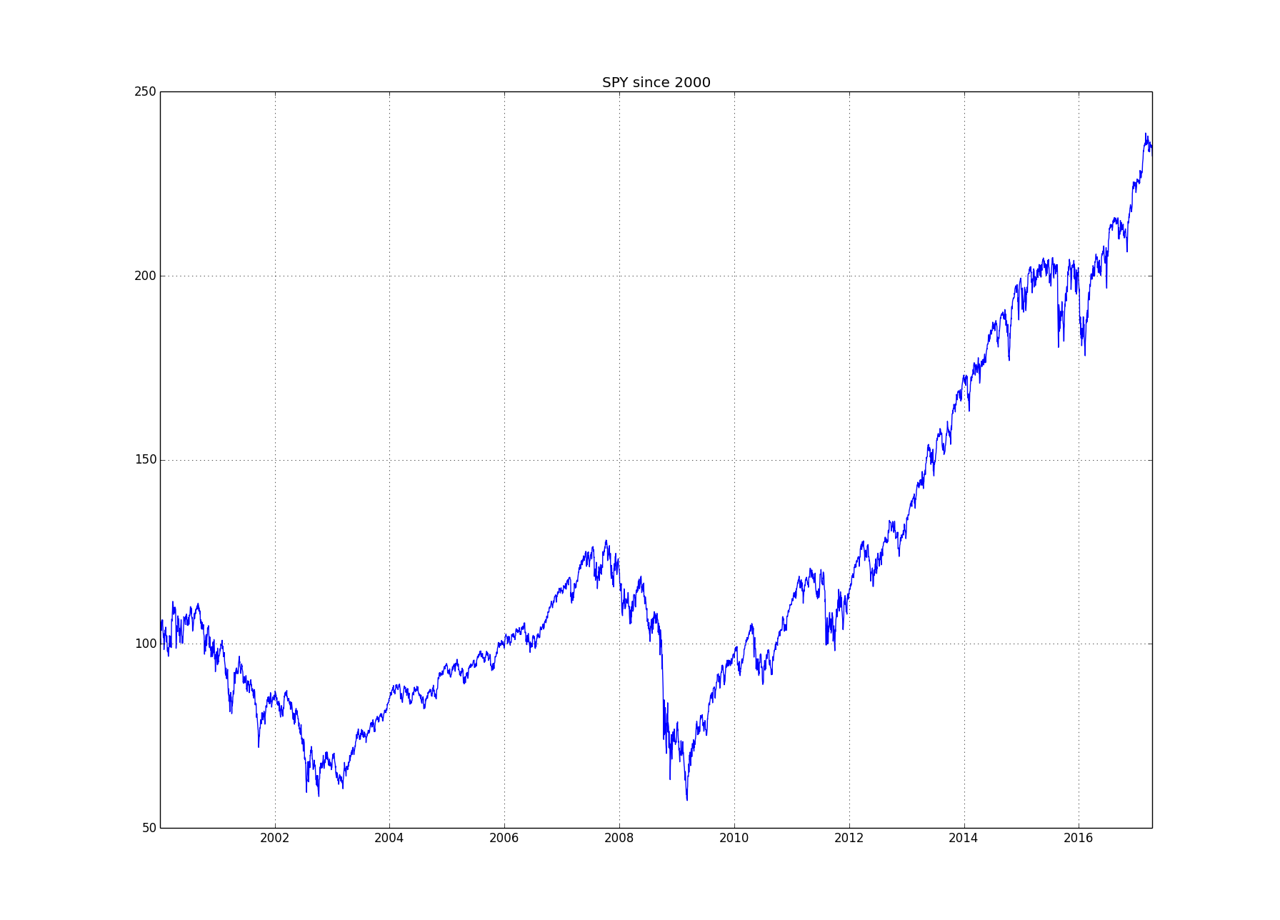
The market seems to have $2$ different regimes:
- A "normal" regime in which the market goes up slowly with little volatility. This regime seems to be present from around $2003$ through $2007$ and most of the period from $2009$ through the present.
- A more rare "crisis" regime in which the market goes down, faster than it goes up in more normal times, and with high volatility. This regime seems to be present from $2000$ until $2003$ and during $2008$.
| state | transition probability | mean | volatility | |
| 1 | 97.8% | 2.2% | -10bps | 196bps |
| 2 | 0.9% | 99.1% | 7bps | 72bps |
This seems to fit all of the stylized facts previously listed, in particular:
- There is a "normal" state (state $2$) which is moving up: the mean return, which corresponds with the slope with respect to time, is positive ($7$bps) and a "crisis" state (state $1$) in which it is moving down: the mean return is negative ($-10$bps).
- The process moves up more slowly than it moves down. In particular, the absolute value of the mean return (slope) of the "normal" state ($7$bps) is less than the absolute value of mean return (slope) of the "crisis" state ($10$bps).
- The volatility of the "normal" state ($72$bps) is less than the volatility of the "crisis" state ($196$bps).
- As calculated when we discussed stationary distributions, the long-term average (stationary probability) of the amount of time spent in the "normal" state (about $71\%$) is more than this quantity for the "crisis" state (about $29\%$).
We now look at whether the timing of when the chain is in the "normal" state versus the "crisis" state matches our intuition. Given any finite sequence of observations from an HMM with an irreducible aperiod underlying Markov chain such as this one, we can never know for sure which state we are in. At any given time, there is a probability that we are in each state given the data that we have seen. We can calculate this probability by: \begin{eqnarray*} \mathbb{P}\left(\left.X_t=s_i\right|Y^t=y^t\right) = \frac{f_\theta{\left(x_t=s_i,y^t\right)}}{f_\theta{\left(y^t\right)}} = \frac{\alpha_t(i)}{\sum_i\alpha_t(i)} \end{eqnarray*} The next chart shows the probability of a normal market superposed with the cumulative return of the market over time:
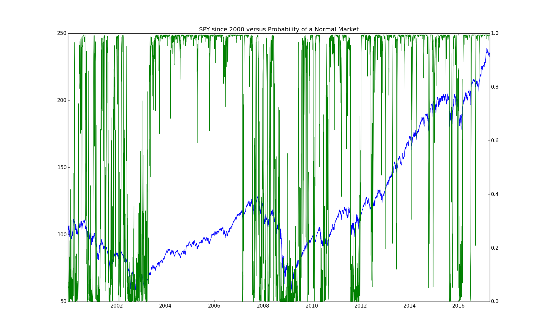
We can see from this chart that the period from $2003$ through $2007$ has a high probability of being in the "normal" state as was our hypothesis. The period from $2009$ through the present is mostly so, as we also hypothesized. The periods before $2003$ and during $2008$ are a bit more mixed than I would have hypothesized but with a tendency towards a low probability of being in the "normal" state.
3 Regime Model
We now investigate whether a $3$ state model has more explanatory power than a $2$ state model of SPY returns. We recall the $3$ state model that we had discussed as an example in the section on stationary distributions:
| state | transition probability | mean | volatility | ||
| 1 | 96.8% | 3.2% | 0.0% | -15bps | 271bps |
| 2 | 0.7% | 96.8% | 2.5% | -3bps | 117bps |
| 3 | 0.0% | 2.5% | 97.5% | 11bps | 55bps |
Note that this model has the same features that were mentioned for the $2$-state model but more strongly if one considers state $1$ as the "crisis" state and state $3$ to be the "normal" state. In addition, there is an "intermediate" state, state $2$ which is somewhere in between "crisis" and "normal" in both mean and volatility. An interesting aspect of this model is that some of the transitions were fit as having $0$ probability (in actually, the probabilities had not converged to $0$ but were so small as to not happen in millions of observations). The graph of the process is:
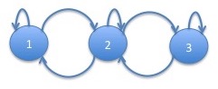
Note that the probability of being in the "crisis" state goes down to about $10\%$. We now plot the cumulative SPY return superposed with the probabilities of the "crisis" and "normal" states:
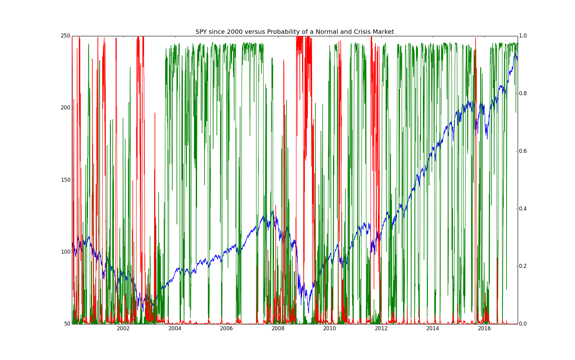
One difference between this chart and the equivalent chart for the $2$-state model is that, in the period from $2000$ until $2003$, the market does not have $100\%$ probability of being in the "normal" state, at least not very often.
4 Regime Model
We now investigate whether a $4$ state model has more explanatory power than a $2$ state model of SPY returns. The parameters of the $4$ state model are given as follows:
| state | transition probability | mean | volatility | |||
| 1 | 95.08% | 4.92% | 0.00% | 0.00% | -28bps | 359bps |
| 2 | 0.70% | 97.66% | 1.64% | 0.00% | -6bps | 157bps |
| 3 | 0.04% | 0.99% | 94.75% | 4.22% | 0bps | 99bps |
| 4 | 0.00% | 0.00% | 3.75% | 96.25% | 11bps | 52bps |
The graph of the Markov chain underlying this HMM is:
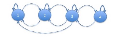
Notice that the linear structure that we saw in the $3$ state chain largely continues in the $4$-state chain. Most of the times, the process progresses from state $4$ to states $3$, $2$ and $1$ getting progressively worse. However, occasionally, the process can jump from state $3$ to state $1$. This happens with probability $0.04\%$ meaning that it would have happened about $1$ or $2$ times in data the size of our $17$ years of observations. Note that there is no corresponding jump upwards. This is consistent with the idea that markets can progress downwards faster than they progress upwards.
The stationary distribution of this transition matrix is given by: \begin{eqnarray*} \left(\begin{array}{cccc}3.4\% & 22.1\% & 35.1\% & 39.4\%\end{array}\right) \end{eqnarray*} The process spends little time in the catastrophic crisis state.
Can we Apply the Log-likelihood Ratio Test between the $2$ and $3$ State Models
Note that the general $2$-state model is nested in the general $3$-state model. The $2$ state model has $m*(m-1)=2$ transition probabilities $2m=4$ parameters from the distributions of the observations for a total of $6$ parameters. The $3$ state model has $6$ transition probabilities $6$ parameters from the distributions of the observations for a total of $12$ parameters. If we set the following parameters in the general $3$ state model: \begin{eqnarray} \pi_1 & = & 1\nonumber\\ p_{1,3} & = & 0\label{to3}\\ p_{3,1} & = & 0\label{from3}\\ p_{2,3} & = & 0\label{from2to3}\\ p_{3,2} & = & 0\label{from3to2}\\ \mu_3 & = & 0\nonumber\\ \sigma_3 & = & 1\nonumber\\ \end{eqnarray} we get the general $2$ state model so that the models are nested as required for the log likelihood ratio test. Note that we are not fiting the initial distribution $\pi$ so we are constraining a total of $6$ parameters that we are fitting above which would be the number of degrees of freedom of a log likelihood ratio test. However, there are a few subtleties in trying to apply the log likelihood ratio test.
Transitions probabilities that were fit as $0$
Notice that when we fit the $3$-state model, some of the transition probabilities were fit as $0$. We first consider the simpler log likelihood ratio test between these parameters be constrained to be $0$ versus no constraints on these parameters. Since the parameters were fit as $0$ without constraints, the likelihood will be exactly the same for the model with and without the constraint. Hence, the log likelihood ratio is $0$. Any test would choose the model with these transitions constrained to be $0$. The transition probabilities which had been fit as $0$ correspond to equations (\ref{to3}) and (\ref{from3}) in the above list. We now proceed to investigate whether the other $4$ constraints required to make the $3$ state model into the $2$ state model will also be accepted by a log likelihood ratio test.
Testing whether transitions probabilities should be $0$
Note that in the presentation on the theorem which indicated that the asymptotic distribution of twice the log likelihood ratio is $\chi^2$, we indicated that there were technical conditions. In this section we discuss why those technical conditions prohibit us from using this result in determining the number of states or structure of an HMM.
The technical conditions include the following:
- The parameter sets $\Theta_0$ and $\Theta_1$ that we are testing must be closed (under limits) and bounded.
- The true parameter $\theta^*$ must not be on the boundary of either $\Theta_0$ or $\Theta_1$.
In this paragraph, we investigate the first requirement above. Notice that the transition probabilities from a given state have the following constraints: \begin{eqnarray*} p_{s_i,s_j} & \geq & 0\\ \sum_j p_{s_i,s_j} & = & 1\\ \end{eqnarray*} This implies that $0\leq p_{s_i,s_j} \leq 1$ and so the transition probabilities are in a bounded set. Neither the means nor standard deviations are bounded. Hence, one condition is that we put minimum and maximum bounds on the means and standard deviations. As mentioned previously, it is helpful to bound the standard deviation above $0$ to keep the likelihood bounded. That is required here as well.
We now look into the second requirement. In order to fit the $2$ state HMM into a $3$ state Markov chain (with $0$ for $p_{1,3}$ and $p_{3,1}$ as mentioned previously), we could add constraints such as (\ref{from2to3}) and (\ref{from3to2}) above. However, this puts the parameters on the boundary of the set of transition probabilities for $3$ state HMM's which means the theorem would not hold in this case. Even if we could make it hold for this case, in testing a $3$ state chain versus a $4$ state chain, we would have similar failures since we are constraining several transition probabilities of the $3$ state chain to be $0$ and hence on the boundary. To quote a book from 2005 "As explained below, refining those consistency and efficiency results requires a precise understanding of the behavior of the likelihood ratios. As of writing of this text, in the HMM setting, this precise picture is beyond our understanding." To my knowledge, this remains the state of affairs. In a future lecture, we will discuss a different approach to deciding on the order of an HMM: the Bayesian approach in which we decide not to make a decision.
References
-
Cappe, Olivier, Moulines, Eric and Ryden, Tobias. Inference in Hidden Markov Models. Springer, 2005.
This is a good book on the statistics of HMM's.
-
Mamon, Rogemar S. and Elliott, Robert J. Hidden Markov Models in Finance, Volume II. Springer, 2014.
This is a book of papers include empirical tests such as the ones done here using HMM's in finance.