Markov Process and Chain
We now begin a more formal study of Markov chains. The first publication on Markov chains was by Russian mathematician A.A. Markov in 1906. Markov's paper was a response to a paper in which his academic nemesis, Nekrasov, claimed to have proved the existence of free will in part using the notion that the law of large numbers only applies to independent random variables. In the first paper, Markov demonstrates that the law of large numbers also applies to dependent events, in particular, to Markov chains. While much of probability and statistics deal with independent random variables, Markov chains are an important class of stochastic processes with dependencies.
A sequence of random variables $X_1, X_2, X_3, \ldots$ has the Markov property if for any $t$, $X_1, X_2, \ldots, X_{t-1}$ and $X_{t+1}$ are conditionally independent given $X_t$. This can be expressed as, for any $t$ and any set $A$: \begin{eqnarray} \mathbb{P}\left(X_{t+1} \in A\right|\left.X_1, X_2, \ldots, X_t\right) = \mathbb{P}\left(X_{t+1}\in A\right|\left. X_t\right)\tag{1}\label{Markov} \end{eqnarray} If we call $t$ the present, any larger time the future and any smaller time the past, the previous property can be stated as "the future is independent of the past given the present".
For our purposes, a Markov chain is a Markovian sequence of random variables taking values in a discrete set called the state space. Note that usage of the term Markov chain is not standardized in the academic literature, often refering to a process which is continuous in time, or even sometimes in space, rather than discrete as we consider here. A finite Markov chain is one in which the state space is finite, which is the object of study of much of this course. We will use the symbols $s, s', s_1, s_2, \ldots$ for variables that represent states of a Markov chain and symbols $t$ for time. For a finite Markov chain, (\ref{Markov}) becomes, for any $t$ and states $s_1, s_2, \ldots, s_{t+1}$: \[ \mathbb{P}\left(X_{t+1}=s_{t+1}\right|\left.X_1 = s_1, X_2=s_2, \ldots, X_t=s_t\right) = \mathbb{P}\left(X_{t+1}=s_{t+1}\right|\left. X_t=s_t\right) \]
While we have defined the Markov property in terms of the conditional distribution of the process at a single time $t+1$, the property automatically extends to the conditional distribution of all times larger than $t$:
\begin{eqnarray} \lefteqn{\mathbb{P}\left(X_{t+1}=s_{t+1}, X_{t+2}=s_{t+2}, \ldots, X_{t+n}=s_{t+n}\right|\left.X_1=s_1, X_2=x_2, \ldots, X_t=s_t\right)}\\ & = & \prod_{i=1}^n \mathbb{P}\left(X_{t+i}=s_{t+i} \right|\left. X_1=s_1, X_2=s_2, \ldots, X_{t+i-1}=s_{t+i-1}\right)\\ & = & \prod_{i=1}^n \mathbb{P}\left(X_{t+i}=s_{t+i} \right|\left. X_{t+i-1}=s_{t+i-1}\right)\\ & = & \prod_{i=1}^n \mathbb{P}\left(X_{t+i}=s_{t+i} \right|\left. X_{t}=s_t, X_{t+1}=s_{t+1}, \ldots, X_{t+i-1}=s_{t+i-1}\right)\\ & = & \mathbb{P}\left(X_{t+1}=s_{t+1}, X_{t+2}=s_{t+2}, \ldots, X_{t+n}=s_{t+n} \right|\left. X_t=s_t\right)\tag{2}\label{future} \end{eqnarray}Hence, if a process is Markovian, the probability distribution of all subsequent values is dependent only upon the most recent value.
Homogeneous Markov Chain
A Markov chain is homogeneous (or, sometimes time invariant) if the conditional probabilities in (\ref{Markov}) are independent of time: \[ \mathbb{P}\left(X_{t+1}=s_{t+1}\right|\left.X_t=s_t\right) = \mathbb{P}\left(X_2=s_{t+1}\right|\left.X_1=s_t\right) \] In this class, we will deal mainly with homogeneous Markov chains. The transition matrix, $P$, of a homogeneous finite Markov chain is defined as: \[ P_{s_t,s_{t+1}} = \mathbb{P}\left(X_{t+1}=s_{t+1}\right|\left.X_t=s_t\right) \] The initial distribution, $\pi$, of the Markov chain is defined as: \[ \pi_s = \mathbb{P}\left(X_1 = s\right) \] For a homogeneous Markov chain, all probabilities can be calculated via the transition matrix and the initial distribution: \begin{eqnarray} \lefteqn{\mathbb{P}\left(X_{t+1} = s_{t+1}, X_t=s_t, \ldots, X_2 = s_2, X_1 = s_1\right)}\\ & = & \prod_{i=0}^t \mathbb{P}\left(X_{i+1}=s_{i+1}\right|\left.X_i=s_i, X_{i-1}=s_{i-1},\ldots,X_2=s_2,X_1=s_1\right)\\ & = & \mathbb{P}\left(X_1=s_1\right)\prod_{i=1}^t \mathbb{P}\left(X_{i+1}=s_{i+1}\right|\left.X_i=s_i\right)\\ & = & \pi_{s_1}\prod_{i=1}^t P_{s_i,s_{i+1}} \end{eqnarray} The transition matrix of a homogeneous Markov chain has all row sums equal to $1$: \[ P e = \sum_{s_2} P_{s_1,s_2} = \sum_{s_2} \mathbb{P}\left(X_2=s_2\right|\left.X_1=s_1\right) = 1 \] where $e$ is the vector consisting of all $1$'s. Also, all elements of the matrix are non-negative since they are probabilities. A matrix with non-negative entries whose rows sum to $1$ is called a stochastic matrix. The initial distribution of a Markov chain is a point mass function. Note that a homogeneous finite Markov chain is equivalent to a pair $(\pi,P)$ consisting of a point mass function $\pi$ and a stochastic matrix $P$: for any such pair there is a homogeneous finite Markov chain and vice versa.
Example: Simple Model of Prepayments and Defaults
We consider the simple model of prepayments and defaults. Let $\tau_C$ be the first time that $X_i$ is not $C$, that is: \begin{eqnarray} \tau_C = \min \left\{n : X_1 = C, \ldots, X_{n-1} = C, X_n \neq C\right\} \end{eqnarray} $\tau_C$ is a random variable called the first exit time of $C$. Note that $\tau_C$ is potentially dependent upon the entire path of the Markov chain: its value might not be known at any fixed finite time $n$. We will use the formulas above to calculate the probability distribution of the first exit time. Let $p_{C,P}$ and $p_{C,D}$ be the probabilities of going from the $C$ (current) state to the $P$ (prepayment) and $D$ (default) states, respectively. First, we calculate the probability that $\tau_C=1$: \begin{eqnarray} \mathbb{P}\left(\tau_C=1\right) = \mathbb{P}\left(X_1\neq C\right) = \sum_{s\neq C}\pi_s = \pi_P + \pi_D \end{eqnarray} Now, for $n> 1$: \begin{eqnarray} \lefteqn{\mathbb{P}\left(\tau_C=n\right)}\\ & = & \mathbb{P}\left(X_1=C, X_2=C, \ldots, X_{n-1}=C, X_n\neq C\right)\\ & = & \mathbb{P}\left(X_1=C, X_2=C, \ldots, X_{n-1}=C, X_n\in\left\{P,D\right\}\right)\\ & = & \pi_C \left(\prod_{i=2}^{n-1} p_{C,C}\right) \left(p_{C,P} + p_{C,D}\right)\\ & = & \pi_C p_{C,C}^{n-2} \left(p_{C,P} + p_{C,D}\right)\\ & = & \pi_C\left(1 - p_{C,P} - p_{C,D}\right)^{n-2} \left(p_{C,P} + p_{C,D}\right) \end{eqnarray} We now condition on $X_1=C$. In this case, for $n\geq 1$: \begin{eqnarray} \lefteqn{\mathbb{P}\left(\tau_C=n\right|X_1=C\left.\right) = \mathbb{P}\left(\tau_C=n\right|\tau_C> 1\left.\right) = \mathbb{P}\left(\tau_C=n\right|\tau_C\neq 1\left.\right)}\\ & = & \frac{\mathbb{P}\left(\tau_C=n\right)}{1 - \mathbb{P}\left(\tau_C=1\right)} = \frac{\pi_C\left(1 - p_{C,P} - p_{C,D}\right)^{n-2} \left(p_{C,P} + p_{C,D}\right)}{1 - \left(\pi_P + \pi_D\right)} = \left(1 - p_{C,P} - p_{C,D}\right)^{n-2} \left(p_{C,P} + p_{C,D}\right) \end{eqnarray} Note that this is a distribution on the discrete variable $n$ of the form $\left(1-p\right) p^{n-2}$ (in this case, $p=1-p_{C,P}-p_{C,P}$). This distribution is called the geometric distribution (note that, here, we have $\tau_C \geq 2$ for the geometric distribution where it is usually $\tau_C \geq 1$. The geometric distribution is the only discrete memoryless distribution, that is, a random variable $N$ has the geometric distribution if it is memoryless: \begin{eqnarray} \mathbb{P}\left(N \geq n+1\right|\left.N \geq n\right) = \mathbb{P}\left(N \geq 2\right|\left.N \geq 1\right) \end{eqnarray} In other words, $N$ represents the length of time of an event for which the probability that it takes another step is independent of the number of steps that it has taken so far. Since for Markov chains, the probability of leaving a state does not depend upon the history of the chain other than the current state, the time to leave a given state is always geometrically distributed for a Markov chain. First exit times for individual Markov chain states are always geometrically distributed.
Multi-step Transition Probabilities
The transition matrix of a homogeneous Markov chain tells us the probability distribution of the chain after a single step passes. In this section, we show how to calculate the conditional probability distribution of a homogeneous Markov chain after several steps have passed, often called the multi-step transition probabilities. We begin with just $2$ steps: \begin{eqnarray} \mathbb{P}\left(X_{t+2} = s_{t+2}\right|\left.X_t=s_t\right) & = & \sum_s \mathbb{P}\left(X_{t+2} = s_{t+2}, X_{t+1}=s\right|\left.X_t=s_t\right)\\ & = & \sum_s \mathbb{P}\left(X_{t+2} = s_{t+2}\right|\left. X_{t+1}=s, X_t=s_t\right) \mathbb{P}\left(X_{t+1}=s\right|\left.X_t=s_t\right)\\ & = & \sum_s \mathbb{P}\left(X_{t+2} = s_{t+2}\right|\left. X_{t+1}=s\right) \mathbb{P}\left(X_{t+1}=s\right|\left.X_t=s_t\right)\\ & = & \left(P P\right)_{s_t,s_{t+2}} = P^2_{s_t,s_{t+2}} \end{eqnarray} where $P P = P^2$ denote the multiplication of the matrix $P$ by itself. The $2$-step transition matrix is the square of the $1$-step transition matrix. This process can be iterated to yield multi-step transition probabilities: \begin{eqnarray} \mathbb{P}\left(X_{t+1} = s_{t+1}\right|\left.X_1=s_1\right) & = & \sum_s \mathbb{P}\left(X_{t+1} = s_{t+1}, X_t=s\right|\left.X_1=s_1\right)\\ & = & \sum_s \mathbb{P}\left(X_{t+1} = s_{t+1}\right|\left. X_t=s, X_1=s_1\right) \mathbb{P}\left(X_t=s\right|\left.X_1=s_1\right)\\ & = & \sum_s \mathbb{P}\left(X_{t+1} = s_{t+1}\right|\left. X_t=s\right) \mathbb{P}\left(X_t=s\right|\left.X_1=s_1\right)\\ & = & \left(P P^{t-1}\right)_{s_1,s_{t+1}} = P^t_{s_1,s_{t+1}} \end{eqnarray} The $t$-step transition matrix is the $1$-step transition matrix to the power $t$. This equation is sometimes referred to as the Chapman-Kolmogorov equation.
Example: Simple Model of Prepayments and Defaults
We again consider the simple model of prepayments and defaults. This time, we calculate the probability that the Markov chain defaults in $n$ steps given that it starts in state $C$. The probability of going from $C$ to $D$ in 2 steps, written $p^{(2)}_{C,D}$ is given by: \begin{eqnarray} p^{(2)}_{C,D} & = & \sum_s p_{C,s}p_{s,D} = p_{C,P} p_{P,D} + p_{C,C} p_{C,D} + p_{C,D} p_{D,D}\\ & = & \left(1 - p_{C,P} - p_{C,D}\right) p_{C,D} + p_{C,D} \end{eqnarray} Similarly, the probability of going from $C$ to $D$ in $n$ steps is: \begin{eqnarray} p^{(n)}_{C,D} & = & \sum_s p^{(n-1)}_{C,s} p_{s,D} = p^{(n-1)}_{C,P} p_{P,D} + p^{(n-1)}_{C,C} p_{C,D} + p^{(n-1)}_{C,D} p_{D,D}\\ & = & p^{(n-1)}_{C,C} p_{C,D} + p^{(n-1)}_{C,D} = p^{(n-1)}_{C,C} p_{C,D} + p^{(n-2)}_{C,C} p_{C,D} + p^{(n-2)}_{C,D}\\ & = & \ldots = \sum_{i=0}^{n-1} p^{(i)}_{C,C} p_{C,D} \end{eqnarray} Note that $p^{(i)}_{C,C} = \left(1 - p_{C,P} - p_{C,D}\right)^i$ and so: \begin{eqnarray} p^{(n)}_{C,D} & = & \sum_{i=0}^{n-1} \left(1 - p_{C,P} - p_{C,D}\right)^i p_{C,D}\\ & = & \frac{1 - \left(1 - p_{C,P} - p_{C,D}\right)^n}{p_{C,P} + p_{C,D}} p_{C,D} \end{eqnarray} Note that as $n\rightarrow\infty$, this goes to $\frac{p_{C,D}}{p_{C,P} + p_{C,D}}$ which is the formula previously discussed for the probability of eventually ending in $D$ when starting from $C$. However, this formula also gives us the probability of ending in $D$ after each step.
Example: Rating Migrations
More complex examples, such as rating migrations can be handled by computer. The following chart shows the probability of default over time for different starting ratings. We'll go over the code to generate this plot in a future lecture.
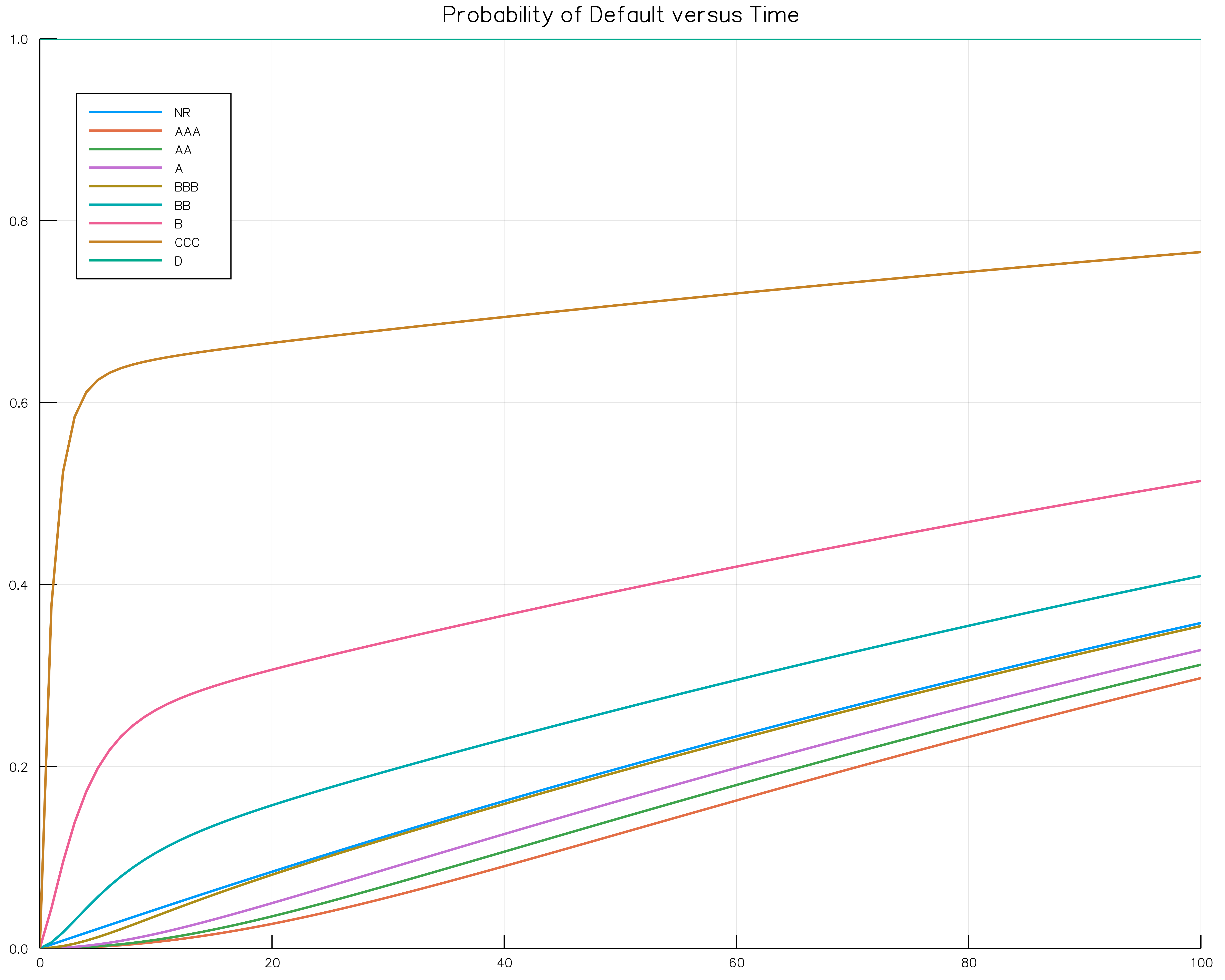
There are a few interesting observations about this chart:
- The non-rated class (NR) is close to the BBB curve. It seems to be roughly where some kind of average of the other curves. The rating agencies purport that ratings are removed from bonds for issues that are not credit related. This is consistent with the non-rated class being an average of the other classes.
- The curves are monotonic in rating as is to be expected.
- In industry, Investment Grade (sometimes just IG) is defined as any bond with rating BBB- or better. While there is a significant difference between IG and non-IG default rates, there is no jump discontinuity here. It seems to be a somewhat arbitrary distinction.
- Most of the ratings seem to become linear in the intermediate time. Note they can't be linear ultimately unless they are flat since probabilities must be between $0$ and $1$. We'll talk about why these curves appear linear later in the course.
Stationary Distributions
A probability distribution is a stationary distribution of a homogeneous Markov chain with stochastic matrix $P$ if: \[ \pi P = \pi\tag{3}\label{stationary} \] If the initial distribution of a homogeneous Markov chain is a stationary distribution, then the (unconditional) distribution of the Markov chain for any period is that same stationary distribution: \begin{eqnarray} \mathbb{P}\left(X_t = s_t\right) & = & \sum_{s_1}\mathbb{P}\left(X_t = s_t\right|\left.X_1=s_1\right) \mathbb{P}\left(X_1 = s_1\right) = \sum_{s_1}P^{t-1}_{s_1,s_t}\pi_{s_1}\\ & = & \left(\pi P^{t-1}\right)_{s_t} = \left(\pi P P^{t-2}\right)_{s_t} = \left(\pi P^{t-2}\right)_{s_t} = \ldots = \pi_{s_t}\\ \end{eqnarray}
We have defined stationary distributions in terms of the system of linear equations (\ref{stationary}). Note that one of these equations is redundant since the rows of the matrix $P$ sum to $1$. To see this, suppose we have $\left(\pi P\right)_s = \pi_s$ for all $s\ne s'$, then: \begin{eqnarray} \left(\pi P\right)_{s'} & = & \sum_s \pi_s P_{s,s'}\\ & = & \sum_s \pi_s \left(1 - \sum_{s''\neq s'} P_{s,s''}\right)\\ & = & \sum_s \pi_s - \sum_s \sum_{s''\neq s'} \pi_s P_{s,s''}\\ & = &\sum_s \pi_s - \sum_{s''\neq s'} \sum_s \pi_s P_{s,s''}\\ & = &\sum_s \pi_s - \sum_{s''\neq s'} \pi_{s''}\\ & = & 1 - \left(1 - \pi_{s'}\right)\\ & = &\pi_{s'} \end{eqnarray} so that the equation also holds for $s'$. We also have the equation $\sum_s\pi_s = 1$ since $\pi$ must be a probability distribution. Does this equation always have a solution? We state the following theorem that says that it does:
Every homogeneous finite Markov chain has a stationary distribution.
Below is an example of the stationary distribution of homogeneous finite Markov chains.
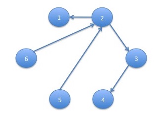
Example: Mortgage Default Model
Consider a homogeneous finite Markov chain corresponding to this graph. We will show that every probability distribution with mass only on states $P$ and $D$ is stationary. Let $\pi = \begin{array}{lllll}\left(\pi_P\right. & 0 & 0 & 0 & \left.\pi_D\right)\end{array}$: \[ \begin{array}{lllll}\left(\pi_P\right. & 0 & 0 & 0 & \left.\pi_D\right)\end{array} \left(\begin{array}{ccccc} 1 & 0 & 0 & 0 & 0\\ p_{C,P} & p_{C,C} & p_{C,30} & 0 & 0\\ 0 & p_{30,C} & p_{30,30} & p_{30,60} & 0\\ 0 & p_{60,C} & p_{60,30} & p_{60,60} & p_{60,D}\\ 0 & 0 & 0 & 0 & 1\\ \end{array}\right) = \begin{array}{lllll}\left(\pi_P\right. & 0 & 0 & 0 & \left.\pi_D\right)\end{array} \] The top and bottom equations become $\pi_P = \pi_P$ and $\pi_D = \pi_D$. Every other equation becomes $0 = 0$. Hence, any such probability distribution is a stationary distribution. In fact, every stationary distribution is of this form since the Markov chain eventually ends up in $P$ or $D$. Hence, a homogeneous finite Markov chain can have multiple stationary distributions. The theorem above says nothing about the uniqueness of stationary distributions.
We now make note of some other things that the theorem does not say:
- A Markov chain with an infinite state space need not have a stationary distribution.
- Even if the stationary distribution is unique, the distribution of the random variables need not converge to the stationary distribution. We will present examples of this as well as go through conditions for uniqueness as well as convergence below. In order to present these conditions, we first introduce some basic language from graph theory in the next section.
We can solve for the stationary distribution by solving a system of linear equations. Similar to absorption probabilities, there is also a method of deriving a stationary distribution of a Markov chain by using graph theory which we present later after more formally defining some terms.
Some Graph Theory Concepts
Graph theory is the study of objects like this graph. A graph is composed of circles called vertices and lines between them called edges. We use the notation $V(G)$ for the set of vertices of a graph $G$ and $E(G)$ for its set of edges. For a set of vertices $V'$ and a set, $E'$, of pairs from $V'$, we will write $G = (V',E')$ for the graph with vertices $V'=V(G)$ and edges $E'=E(G)$. Graphs in which the edges have a direction to them are called directed graphs. For directed graphs, an edge $e\in E(G)$ is an ordered pair of vertices, $(u,v)$, such that $u\in V(G)$ and $v\in V(G)$ and is drawn as an arrow from $u$ to $v$. We call the edge $(u,v)$ an outgoing edge from $u$ and an incoming edge to $v$.
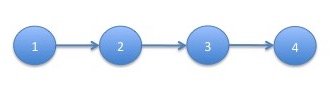
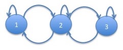
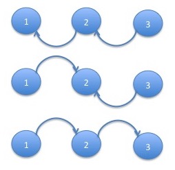
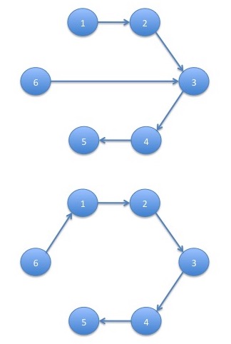
A directed graph $G'$ is a subgraph of a graph $G$, written $G'\subseteq G$ if $V(G') \subseteq V(G)$ and $E(G') \subseteq E(G)$. When $G'\subseteq G$, we say that $G$ contains $G'$. A directed graph for which $V(G)=\left\{u_1, u_2, \ldots, u_n\right\}$ with $u_i \neq u_j$ for $i\neq j$ and $E(G)=\left\{(u_1,u_2),(u_2,u_3),\ldots,(u_{n-1},u_n)\right\}$ is called a path from $u_1$ to $u_n$ or just a path. The following graph is a path:
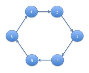
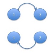
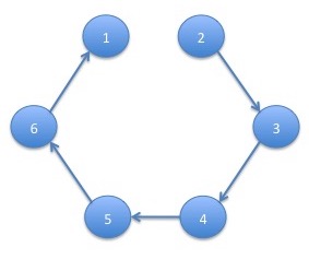
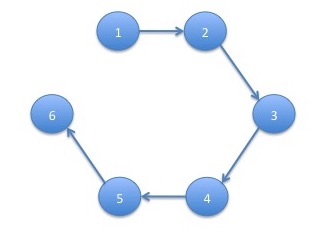
A directed graph for which $V(G)=\left\{u_1, u_2, \ldots, u_n\right\}$ with $u_i \neq u_j$ for $i\neq j$ and $E(G)=\left\{(u_1,u_2),(u_2,u_3),\ldots,(u_{n-1},u_n),(u_n,u_1)\right\}$ is called a cycle. A cycle returns to where it started whereas a path does not. The following graph is a cycle:
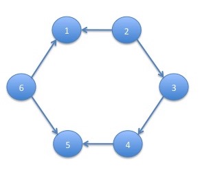
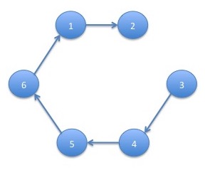
The out-degree of a vertex $v\in V(G)$, written, $d_G(v)$ is the number of outgoing edges from $v$. For example, in a cycle, $G$, we have that $d_G(v) = 1$ for all $v\in V(G)$. An undirected path or an undirected cycle is a path or cycle in which the edges can go in either direction. More precisely, an undirected path is a graph $G$ such that $V(G) = \left\{u_1,u_2,\ldots,u_n\right\}$ such that $u_i\neq u_j$ for $i\neq j$ and, for all $i\lt n$, either $\left(u_i,u_{i+1}\right)\in E(G)$ or $\left(u_{i+1},u_i\right)\in E(G)$. An undirected cycle is defined similarly. The graph below is an example of a undirected cycle:
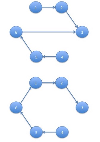
A graph is connected if, for any $u,v\in V(G)$, there is an undirected path between $u$ an $v$. Finally, a graph is a tree if it connected and has no undirected cycles. The graph below is an example of a tree:
The Graph of a Markov Chain
The graph of a Markov chain is the graph in which the vertices are the states of the Markov chain and the edges are the pairs of states, $(s,s')$, which have non-zero transition probability, that is, $P_{s,s'}>0$.
Example: the Absorption Probability Formula
As an example of the use of graph theory, we now give a more concise version of the combinatorial formula for the absorption probabilities that we gave in the last lecture. Let $G$ be the graph of a Markov chains with absorbing states $A\subseteq V(G)$. Let $F(G)$ be the set of all subgraphs, $G'\subseteq G$ which contain no cycles and such that every non-absorbing vertex has exactly one outgoing edge, that is, $d_{G'}(v)=1$ for all $v\in V(G') - A$. For any $s\in V(G)$ and $s'\in A$, let $F_{s,s'}(G)$ be the subset of $F(G)$ such that there is a path from $s$ to $s'$. The probability of eventually ending up in state $s'$ when starting in state $s$ is given by: \[ q_{s,s'} = \frac{\sum_{G'\in F_{s,s'}(G)}\prod_{(u,v)\in E(G')} p_{u,v}}{\sum_{G'\in F(G)}\prod_{(u,v)\in E(G')} p_{u,v}} \]
Communicating Classes and Recurrence
For a Markov chain, we say that state $s$ leads to state $s'$, written $s\rightarrow s'$ if there is a path from $s$ to $s'$ in the graph of the Markov chain. We say that state $s$ and $s'$ of a Markov chain communicate, written $s \leftrightarrow s'$ if $s\rightarrow s'$ and $s'\rightarrow s$. A set of states, $C$, of a Markov chain is a communicating class if:
- For all $s,s'\in C$, we have $s\leftrightarrow s'$
- If $s\in C$ and $s\leftrightarrow s'$ then $s'\in C$
A state $s$ of a Markov chain is said to be recurrent if it occurs again, given that it occurs once, with probability $1$. A recurrent state occurs an infinite number of times, if it occurs at all, with probability $1$ since it will repeatedly occur. A state which is not recurrent is called transient. A transient state occurs a finite number of times. Recurrence (and hence transience) is a class phenomenon: if some $s\in C$ is recurrent then so is every $s'\in C$. Hence, we will refer to classes as recurrent or transient.
If a recurrent communicating class contains a single state, that state is an absorbing state. If a Markov chain contains only a single communicating class, it is called irreducible.
The Markov Chain Tree Theorem
Similar to the formula for the absorption probabilities of a Markov chain, there is a combinatorial formula for the stationary distribution. This result is called the Markov chain tree theorem. In order to state it, we introduce a special set of subraphs of a graph $G$ given a vertex $s\in V(G)$. Let $T_s(G)$ be the set of all subgraphs $G' \subseteq G$ such that:
- $V\left(G'\right) = V(G)$
- $v\rightarrow s$ for all $v\in V\left(G'\right)$
- $d_{G'}(v) = 1$ for all $v\in V\left(G'\right) - \{s\}$
- $d_{G'}(s) = 0$
For any irreducible Markov chain with graph $G$ and stochastic matrix $P$, the unique stationary distribution of the Markov chain, denoted by $\pi$, is given by: \begin{eqnarray} \pi_s = \frac{\sum_{G'\in T_s(G)}\prod_{(u,v)\in E(G')} p_{u,v}}{\sum_s\sum_{G'\in T_s(G)}\prod_{(u,v)\in E(G')} p_{u,v}}\tag{4}\label{Markovtree} \end{eqnarray}
It can be shown that the subgraphs of $T_s(G)$ are trees hence the name Markov chain tree theorem. The result has been derived by many people independently. David Aldous, a famous probabalist, has called the Markov chain tree theorem the most rederived result in history. However, I believe there is a reason for it: the result is one that people consider important but is not widely taught.
In order to prove this result, we need to define a another set of subgraphs of a graph $G$: \begin{eqnarray*} C_s(G) = \left\{G' = \left(V(G),E'\right) \subseteq G: v \rightarrow s \mbox{ and } d_{G'}(v) = 1 \mbox{ for all $v\in V(G)$}\right\} \end{eqnarray*} When we add an edge from $s$ to some $v$ for an element of $T_s(G)$, we get an element of $C_s(G)$. In fact, this operation is a one to one correspondence which will be important later. A one to one correspondence (also called a bijection) is a function, $f:A\rightarrow B$, with the following properties:
- The function is one to one (also called an injection) if $f(a) = f\left(a'\right)$ implies that $a = a'$.
- The function is onto (also called an surjection) if for all $b\in B$, there is an $a\in A$ such that $f(a)=b$.
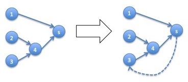
The transformation $f_s:V(G) \times T_s(G) \rightarrow C_s(G)$ given by: \begin{eqnarray*} f_s( v, T ) = \left( V(T), E(T) \cup \left\{(s,v)\right\}\right) \end{eqnarray*} is a one to one correspondence.
The importance of this transformation is that it will correspond with multiplying the stationary distribution at $s$, that is $\pi_s$, by $p_{s,v}$. This transformation can be visualized by the following diagram:
We need to show the following:
- In order for the function have the indicated range, we need to have $f_s(v,T)\in C_s(G)$
- For the function to be one to one, we need that $f_s(v,T) = f_s(v',T')$ implies that $v=v'$ and $T=T'$
- For the function to be onto, we need that for all $G'\in C_s(G)$, there is a $v\in V(G)$ and a $T\in T_s(G)$ such that $f_s(v,T) = G'$
- $\mathbf{f_s(v,T)\boldsymbol{\in} C_s(G)}$: Let $G'=f_s(v,T)$. Since $T\in T_s(G)$, we have that $d_T(v) = 1$ for $v\in V(G) - \{s\}$. Since $G'$ only adds the edge $(s,v)$ to $T$, that means that $d_{G'}(v) = 1$ for all $v\in V(G)$. The other requirements for $G'\in C_s(G)$ follow similarly.
- $\mathbf{f_s(v,T) = f_s(v',T')}$ implies $\mathbf{v=v'}$ and $\mathbf{T=T'}$: After the transformation, we can delete the unique outgoing edge from $s$ to get back $T$, so that we must have $T=T'$. Similarly, the node that that edge must be $v$ so that $v=v'$.
- For all $\mathbf{G'\boldsymbol\in C_s(G)}$, there is a $\mathbf{v\boldsymbol\in V(G)}$ and a $\mathbf{T\boldsymbol\in T_s(G)}$ such that $\mathbf{f_s(v,T) = G'}$: Here, we have to show that when we delete the unique outgoing edge from $s$, the resulting graph is always an element of $T_s(G)$. Let $T$ be the graph resulting from deleting the outgoing edge form $s$, which we denote by $(s,v)$. Since $d_{G'}(u) = 1$ for all $u\in V(G)$, we have, after we delete the edge $(s,v)$, that $d_T(u)=1$ for all $u\in V(G) - \{s\}$. Furthermore, since $u\rightarrow s$ in $G'$ for all $u\in V(G)$, it must be that $u\rightarrow s$ in $T$ since a path from $u$ to $s$ could not involve the edge $(s,v)$ or it would have a cycle (it would leave $s$ and end in $s$).
There is another operation that takes a vertex $v\in V(G)$ and a tree $T\in T_v(G)$ and yields a graph $G'\in C_s(G)$ by adding the edge $(v,s)$: \begin{eqnarray*} g_s(v,T) = \left(V(T), E(T) \cup \left\{\left(v,s\right)\right\}\right) \end{eqnarray*} That operation is demonstrated by the diagram below:
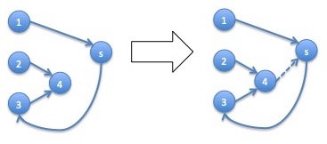
This operation is also a one to one correspondence between the appropriate sets but we don't not show it here.
We now prove the Markov chain tree theorem. The stationary distribution $\pi$ solves the equation: \begin{eqnarray*} \pi P = \pi \end{eqnarray*} that is, $\pi$ is an eigenvector corresponding to eigenvalue $1$. For any eigenvector $v$ corresponding to eigenvalue $\lambda$ of a matrix $M$ and any scalar $\alpha$, the scalar product $\alpha v$ is also an eigenvector corresponding to the eigenvalue $\lambda$: \begin{eqnarray*} (\alpha v) M = \alpha (v M) = \alpha (\lambda v) = (\alpha \lambda) v = \lambda (\alpha v) \end{eqnarray*} Hence, if we define $\tilde{\pi}$ as follows: \begin{eqnarray*} \tilde{\pi}_s = \sum_{G'\in T_s(G)}\prod_{(u,v)\in E(G')} p_{u,v}\tag{5}\label{unnormalized} \end{eqnarray*} then $\tilde{\pi}$ is an eigenvector of $P$ corresponding to eigenvalue $1$ if and only if (\ref{Markovtree}) holds since the denominator of (\ref{Markovtree}) is a scalar. We demonstrate that $\tilde{\pi} P = \tilde{\pi}$ for each state $s$: \begin{eqnarray*} (\tilde{\pi} P)_s & = & \sum_{s'} \tilde{\pi}_{s'} p_{s',s}\\ & = & \sum_{s'} \left(\sum_{G'\in T_s(G)}\prod_{(u,v)\in E(G')} p_{u,v}\right) p_{s',s}\\ & = & \sum_{s'} \sum_{G'\in T_{s'}(G)}p_{s',s} \prod_{(u,v)\in E(G')} p_{u,v}\\ & = & \sum_{s'} \sum_{G'\in T_{s'}(G)} \prod_{(u,v)\in \left(E(G') \cup \left\{(s',s)\right\}\right)} p_{u,v}\\ & = & \sum_{s'} \sum_{G'\in T_{s'}(G)} \prod_{(u,v)\in E(g_s(s',G'))} p_{u,v}\\ & = & \sum_{G'\in C_s(G)} \prod_{(u,v)\in E(G')} p_{u,v}\\ & = & \sum_{s'} \sum_{G'\in T_s(G)} \prod_{(u,v)\in E(f_s(s',G'))} p_{u,v}\\ & = & \sum_{s'} \sum_{G'\in T_s(G)} \prod_{(u,v)\in \left(E(G') \cup \left\{(s,s')\right\}\right)} p_{u,v}\\ & = & \sum_{s'} \sum_{G'\in T_s(G)} p_{s,s'} \prod_{(u,v)\in E(G')} p_{u,v}\\ & = & \sum_{s'} p_{s,s'} \sum_{G'\in T_s(G)} \prod_{(u,v)\in E(G')} p_{u,v}\\ & = & \sum_{G'\in T_s(G)} \prod_{(u,v)\in E(G')} p_{u,v} = \tilde{\pi}_s \end{eqnarray*} where we have used the fact that both $g_s$ and $f_s$ are one to one correspondences.
Example: Regime-switching Market Models
We consider a model of the SPY ETF which tracks the S&P 500 stocks. In this model, the market switches between regimes. In each regime, the market returns are assumed to be lognormal with a different mean and variance. Each regime can switch to another regime with a certain probabilities, making the regimes a Markov chain. Note that these regimes are hidden to us: there are no direct observation of which regime we are in at any point in time. In a later lecture, we will provide detail on how to fit such models.
Example: 2 Regime Model
Consider a $2$ regime model, that is, a model in which the regimes are a $2$-state Markov chain, that is, a Markov chain with the following graph:
We statistically fit this data on the SPY ETF on the portfolio of S&P 500 stocks since it's inception in 1993. The resulting model has the following parameters:
| state | transition probability | mean | volatility | |
| 1 | 97.8% | 2.2% | -10bps | 196bps |
| 2 | 0.9% | 99.1% | 7bps | 72bps |
Note that bps refers to basis points which represents the dimensionless quantity 1/10,000th. A basis point is a percent of a percent and is used widely in finance. In this model, the first state has negative mean return and the second state has positive mean return. The first state also has higher volatility than the second state. This captures stylized facts about the stock market returns such as the association of downward markets with higher volatility and the greater speed of downward movements. We will discuss these stylized facts further in a later lecture. For now, we use the Markov chain tree theorem to derive the stationary distribution. The trees of the graph of this Markov chain are:
The formula for the stationary distribution is then: \[ \pi_1 = \frac{p_{2,1}}{p_{2,1} + p_{1,2}} \approx \frac{0.9\%}{2.2\% + 0.9\%} \approx 29\%\\ \pi_2 = \frac{p_{1,2}}{p_{2,1} + p_{1,2}} \approx \frac{2.2\%}{2.2\% + 0.9\%} \approx 71\%\\ \] Assuming the Markov chain converges to its stationary distribution, which we will hear more about later, the market will spend more than twice as much time in the state which is slowly moving up state than in the state which is volatile and rapidly moving down in the long run.
Example: 3 Regime Model
We now consider fitting a model with $3$ regimes. The resulting model has the following parameters:
| state | transition probability | mean | volatility | ||
| 1 | 96.8% | 3.2% | 0.0% | -15bps | 271bps |
| 2 | 0.7% | 96.8% | 2.5% | -3bps | 117bps |
| 3 | 0.0% | 2.5% | 97.5% | 11bps | 55bps |
Similar to the previous example, the first state has negative returns and the third state positive returns and lower volatility. The middle state is intermediate between the two, both in mean and volatility. For this model, some of the transition probabilities came out as $0$ in the fitting. The chain is only able to move between the first and third states by going through the intermediate state. The graph of this Markov chain is:
The trees of the graph of this Markov chain are:
The formula for the stationary distribution is then: \[ \pi_1 = \frac{p_{3,2}p_{2,1}}{p_{3,2}p_{2,1} + p_{3,2}p_{1,2} + p_{1,2}p_{2,3}} \approx \frac{2.5\% 0.7\%}{2.5\% 0.7\% + 2.5\%3.2\% + 3.2\%2.5\%}\approx 9.8\%\\ \pi_2 = \frac{p_{3,2}p_{1,2}}{p_{3,2}p_{2,1} + p_{3,2}p_{1,2} + p_{1,2}p_{2,3}} \approx \frac{2.5\% 3.2\%}{2.5\% 0.7\% + 2.5\%3.2\% + 3.2\%2.5\%}\approx 45.1\%\\ \pi_2 = \frac{p_{3,2}p_{1,2}}{p_{3,2}p_{2,1} + p_{3,2}p_{1,2} + p_{1,2}p_{2,3}} \approx \frac{3.2\% 2.5\%}{2.5\% 0.7\% + 2.5\%3.2\% + 3.2\%2.5\%}\approx 45.1\%\\ \]
A More Complicated Example of the Markov Chain Tree Theorem: GCD $2$
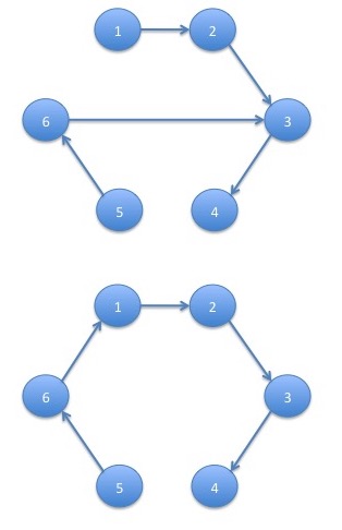
We present one further example of calculating the stationary distribution using the Markov chain tree theorem. We will call the example GCD $2$ for reasons we will discuss later. The graph of the Markov chain is:
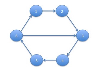
We will make $p_{6,1} = p_{6,3} = \frac{1}{2}$. All other vertices have only a single outgoing edge and the probabilities associated with these edges are $1$. Note that the Markov chain is irreducible.
We consider the set $T_1(G)$ of trees for which the out degree of every vertex other than state $1$ is $1$ and the out degree of state $1$ is $0$. The only vertex for which there are multiple edges to choose is state $6$. If we were to choose the edge $(6,3)$, then since we must choose the edges $\left\{(3,4), (4,5), (5,6)\right\}$ in order for states $4$, $5$ and $6$ to have out degree $1$, we would have a cycle. Hence, the only possibility is to choose $(6,1)$. Hence, the only trees for state $1$ is:
The product of the transition probabilities for this graph is: \[ p_{2,3}p_{3,4}p_{4,5}p_{5,6}p_{6,1} = 1 \cdot 1 \cdot 1 \cdot 1 \cdot \frac{1}{2} = \frac{1}{2} \] The same argument holds for state $2$ which has tree:
and product: \[ p_{1,2}p_{3,4}p_{4,5}p_{5,6}p_{6,1} = 1 \cdot 1 \cdot 1 \cdot 1 \cdot \frac{1}{2}= \frac{1}{2} \] For state $3$, it is possible for either $(6,3)$ or $(6,1)$ to be present:
The sum of the products of the transition probabilities corresponding to these trees is: \[ p_{1,2}p_{2,3}p_{4,5}p_{5,6}p_{6,3} + p_{1,2}p_{2,3}p_{4,5}p_{5,6}p_{6,1} = 1 \cdot 1 \cdot 1 \cdot 1 \cdot \frac{1}{2} + 1 \cdot 1 \cdot 1 \cdot 1 \cdot \frac{1}{2} = 1 \] The same holds for state $4$:
with sum of products: \[ p_{1,2}p_{2,3}p_{3,4}p_{5,6}p_{6,3} + p_{1,2}p_{2,3}p_{3,4}p_{5,6}p_{6,1} = 1 \cdot 1 \cdot 1 \cdot 1 \cdot \frac{1}{2} + 1 \cdot 1 \cdot 1 \cdot 1 \cdot \frac{1}{2} = 1 \] and state $5$:
with sum of products: \[ p_{1,2}p_{2,3}p_{3,4}p_{4,5}p_{6,3} + p_{1,2}p_{2,3}p_{3,4}p_{4,5}p_{6,1} = 1 \cdot 1 \cdot 1 \cdot 1 \cdot \frac{1}{2} + 1 \cdot 1 \cdot 1 \cdot 1 \cdot \frac{1}{2} = 1 \] For state $6$ there are no choices since this is the only state that has multiple outgoing edges:
The product of transition probabilities for this tree is: \[ p_{1,2}p_{2,3}p_{3,4}p_{4,5}p_{5,6} = 1\cdot 1\cdot 1\cdot 1\cdot 1 = 1 \] Taking the sums for each tree over the sum for all trees gives us the stationary probability distribution: \[ \pi_1 = \frac{0.5}{0.5 + 0.5 + 1 + 1 + 1 + 1} = \frac{1}{10}\\ \pi_2 = \frac{0.5}{0.5 + 0.5 + 1 + 1 + 1 + 1} = \frac{1}{10}\\ \pi_3 = \frac{1}{0.5 + 0.5 + 1 + 1 + 1 + 1} = \frac{2}{10}\\ \pi_4 = \frac{1}{0.5 + 0.5 + 1 + 1 + 1 + 1} = \frac{2}{10}\\ \pi_5 = \frac{1}{0.5 + 0.5 + 1 + 1 + 1 + 1} = \frac{2}{10}\\ \pi_6 = \frac{1}{0.5 + 0.5 + 1 + 1 + 1 + 1} = \frac{2}{10}\\ \]
Periodicity and Convergence
Starting from an arbitrary initial distribution, what can we say about the eventual distribution to which a homogeneous finite Markov chain converges? It is not hard to demonstrate that, if a homogeneous Markov chain converges to any distribution, it will converge to a stationary distribution. An irreducible homogeneous finite Markov chain has a unique stationary distribution. Starting from any initial distribution, will the Markov chain converge to the stationary distribution? Under conditions, the answer to this will be yes. However, there are Markov chains for which the answer to this question is no as demonstrated by the following examples.
Example: A $2$-Cycle
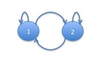
We now demonstrate a Markov chain which does not in general converge to a stationary distribution. Consider a Markov chain corresponding to the following graph:
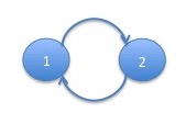
Note that since each state has only a single outgoing edge, the probability associated with both edges is $1$. Starting in the initial distribution $\begin{array}{ll}( 1 & 0 )\end{array}$ the probability distribution of the chain will evolve as follows: \[ \begin{array}{ll} ( 1 & 0 )\\ ( 0 & 1 )\\ ( 1 & 0 )\\ ( 0 & 1 )\\ \end{array}\\ \ldots \] This Markov chain is irreducible and so has a unique stationary distribution. The unique stationary distribution is $\begin{array}{ll}( 0.5 & 0.5 )\end{array}$. The Markov chain will stay in this stationary distribution if started in it. However, the chain will not converge to this stationary distribution given any initial distribution other than the stationary distribution itself.
This example can be modified to be a cycle of length $3$:
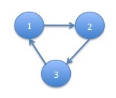
or any other length.
Example: GCD $2$
In the last example, we demonstrated a $2$-cycle. In this example, we provide an example which doesn't contain a $2$-cycle but for which there are some distributions between which the evolution alternates. This is the example that we previously referred to as GCD $2$ whose graph is given here. Starting with the initial distribution: \[ \begin{array}{llllll}( 0.2 & 0.0 & 0.4 & 0.0 & 0.4 & 0.0 )\end{array} \] the probability distribution of the chain will evolve as follows: \[ \begin{array}{llllll} ( 0.2 & 0.0 & 0.4 & 0.0 & 0.4 & 0.0 )\\ ( 0.0 & 0.2 & 0.0 & 0.4 & 0.0 & 0.4 )\\ ( 0.2 & 0.0 & 0.4 & 0.0 & 0.4 & 0.0 )\\ ( 0.0 & 0.2 & 0.0 & 0.4 & 0.0 & 0.4 )\\ \end{array}\\ \ldots \] The behavior of the chain on this initial distribution is the same as in the previous example: it alternates between $2$ distributions. Note that the Markov chain will converge to a limit cycle, that is, it will always converge to situation where it alternates between $2$ distributions. However, unlike in the last example, which will alternate between the initial distribution and a shifted initial distribution, this chain will, in general, change over time until it approaches a limit cycle.
Periodicity
Periodicity is the key property which will help us describe the convergence of irreducible homogeneous finite Markov chains. Periodicity is a graph-theoretic concept: the period of an irreducible Markov chain is the greatest common divisor of the number of vertices in each of its directed cycles. Note that the period is a communicating class property: it is the same for all states in a given communicating class. Hence, for an irreducible Markov chain, the period is the same for all states. If the period $d=1$, the chain is called aperiodic.
The Period of GCD $2$ is $2$
In this example, we show that the period of the Markov chain which we have been calling GCD $2$ is $2$. The cycles of this Markov chain are the one with $V(G') = \left\{1,2,3,4,5,6\right\}$ and the one with $V(G')=\left\{3,4,5,6\right\}$. The number of vertices of these cycles are $4$ and $6$ with greatest common denominator $2$ so the period of this Markov chain is $2$. Note that there is also an undirected cycle with $V(G')=\left\{1,2,3,6\right\}$ but we do not count these here.The Perron-Frobenius Theorem
The celebrated Perron-Frobenius theorem, published in 1907 and 1912, will take us a long way towards answering questions of convergence for stationary distributions of Markov chains. We state the theorem for stochastic matrices. Note that irreducibility and periodicity are properties of the stochastic matrix of the Markov chain. Recall that a left eigenvector of a real matrix $P$ is a vector $l$ for which $l P = \lambda l$ for some $\lambda$ and a right eigenvector $r$ is one for which $P r = \lambda r$ for some $\lambda$. An eigenvalue of a matrix $P$ is simple if it occurs as a root of multiplicity $1$ in the polynomial defined by $\det\left(P - \lambda I\right)$ where $\det$ denotes the determinant.
For any irreducible stochastic matrix, $P$, with period $d$:
- Each of the $d$ roots of unity, that is $\exp\left(\frac{2\pi i j}{d}\right)$ where $i=\sqrt{-1}$ and $j\in\left\{0,\ldots,d-1\right\}$, is a simple eigenvalue of $P$.
- For any eigenvalue $\lambda$ other than those listed above, $\left|\lambda\right| < 1$.
- Only eigenvectors corresponding to the eigenvalue $1$ (the $0$th root of unity) can be chosen to be positive.
We now use the Perron-Frobenius theorem to show that an irreducible finite homogeneous Markov chain converges geometrically to a limit cycle of the periodicity of the chain. We will do this in the slightly limited context of a diagonalizable matrix.
Let $P$ be the stochastic matrix of an irreducible homogeneous finite Markov chain with period $d$ and initial distribution $\pi_0$. Let $\pi^*$ be the unique stationary distribution of $P$ (we use $\pi^*$ because we will use $\pi$ as the circumference of a circle with unit diameter in the proof). There are probability distributions $\pi_1, \ldots, \pi_d$ such that $\frac{1}{n}\sum_{j=1}^d\pi_j = \pi^*$ and for each $j\in\left\{1,\ldots,d\right\}$: \[ \lim_{n\rightarrow\infty}\pi_0P^{nd + j} = \pi_j \] and the convergence is geometric, that is, $\left\|\pi_j - \pi_0 P^{nd+j}\right\| < \alpha\beta^n$ for some $\alpha\in[0,\infty)$ and $\beta\in[0,1)$. If $d=1$ then $\pi_1 = \pi^*$.
We prove this for the case in which $P$ is diagonalizable. The result could be proved when $P$ is not diagonalizable using the somewhat more technical machinery of the Jordan normal form.
Let $\lambda_0, \ldots, \lambda_{n-1}$ be the eigenvalues, $l_0, \ldots, l_{n-1}$ the left eigenvectors. Since $P$ is diagonalizable, we have that $\pi_0 = \sum_{k=0}^{n-1} \alpha_k l_k$. Now, for any $j\in\left\{1,\ldots,d\right\}$: \begin{eqnarray} \pi_0P^{nd+j} & = & \sum_{k=0}^{n-1}\alpha_k l_k P^{nd+j} = \sum_{k=0}^{n-1}\alpha_k \lambda_k^{nd+j}l_k = \sum_{k=0}^{d-1}\alpha_k \exp\left(\frac{2\pi ik}{d}\right)^{nd+j}l_k + \sum_{k=d}^{n-1}\alpha_k\lambda_k^{nd+j}l_k\\ & = & \sum_{k=0}^{d-1}\alpha_k \exp\left(2\pi i n k + \frac{2\pi i j k}{d}\right)l_k + \sum_{k=d}^{n-1}\alpha_k\lambda_k^{nd+j}l_k = \sum_{k=0}^{d-1}\alpha_k \exp\left(\frac{2\pi i j k}{d}\right)l_k + \sum_{k=d}^{n-1}\alpha_k\lambda_k^{nd+j}l_k\\ \end{eqnarray} Now note that $\left|\lambda_k\right|<1$ for $k\in \left\{d,\ldots,n-1\right\}$ from the Perron-Frobenius theorem so that $\lim_{n\rightarrow\infty}\lambda_k^{nd+j} = 0$. Hence: \begin{eqnarray} \lim_{n\rightarrow\infty}\pi_0P^{nd+j} & = & \lim_{n\rightarrow\infty}\sum_{k=0}^{d-1}\alpha_k \exp\left(\frac{2\pi i j k}{d}\right)l_k + \lim_{n\rightarrow\infty}\sum_{k=d}^{n-1}\alpha_k\lambda_k^{nd+j}l_k = \sum_{k=0}^{d-1}\alpha_k \exp\left(\frac{2\pi i j k}{d}\right)l_k \end{eqnarray} Naming the right hand side $\pi_j$ gives (\ref{limit}).
We now show that $\sum_i \pi_j = \pi^*$. \begin{eqnarray*} \lefteqn{\frac{1}{d}\sum_{j=1}^d\sum_{k=0}^{d-1}\alpha_k \exp\left(\frac{2\pi ijk}{d}\right)l_k}\\ & = & \frac{1}{d}\sum_{k=0}^{d-1}\sum_{j=1}^d\alpha_k \exp\left(\frac{2\pi ijk}{d}\right)l_k\\ & = & \frac{1}{d}\sum_{k=0}^{d-1}\alpha_k \left(\sum_{j=0}^{d-1}\exp\left(\frac{2\pi ijk}{d}\right)\right)l_k\\ \end{eqnarray*} But, we have: \begin{eqnarray*} \sum_{j=0}^{d-1}\exp\left(\frac{2\pi ijk}{d}\right) = \left\{\begin{array}{ll} \frac{1 - 1}{1 - \exp\left(\frac{2\pi ik}{d}\right)}=0 & \mbox{if $k\neq 0$}\\ d & \mbox{otherwise}\\ \end{array}\right. \end{eqnarray*} Hence: \begin{eqnarray*} \frac{1}{d}\sum_{j=1}^d\sum_{k=0}^{d-1}\alpha_k \exp\left(\frac{2\pi ijk}{d}\right)l_k = \frac{1}{d} d l_0 = l_0 \end{eqnarray*} Note that $l_0$ is the only positive eigenvector, from the Perron-Frobenius theorem and is the only eigenvector which corresponds to an eigenvalue $1$. The stationary distribution $\pi^*$ is also an eigenvector corresponding to eigenvalue $1$. Hence, $\pi^*=l_0$ which shows the second part of the theorem.
Geometric convergence is very fast. For example for the Markov chain that we called GCD 2, we have that $\beta\approx 0.84$ and $\alpha\le 6$ so that, after $100$ steps, the difference between the distribution and the stationary distribution is less than $10^{-6}$.
Example: Fully General Dynamics of Finite Homogeneous Markov Chains
The graph below indicates the full generality of the behavior of homogeneous finite Markov chains.
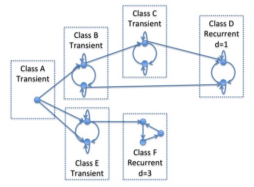
We assume that the initial distribution puts all probability in the state in communicating class A. The Markov chain spends some time in transient communicating classes but will eventually end up in one of the recurrent classes where it will remain. Communicating class A is transient. In fact, the chain will leave class A after $1$ step, entering either class B or class E. If it enters class B, it might remain for some time since this class has cycles. However it will eventually leave to enter either class C or class D. If it enters class C, it might again remain for some time but will ultimately end up in class D. Class D is recurrent so that, if the Markov chain enters this class, it will remain there indefinitely. The class also has period $d=1$ which means that the distribution of the chain will eventually converge to the unique stationary distribution of the class. If the chain leaves class A through class E rather than B, it might remain there for some time but will eventually proceed to class F since class E is transient. Note that, if it enters class E through the state which is lower in the diagram, it will be in class E for at least 2 steps since it can't enter class F from that state. Finally, the chain will end in class F which is recurrent and so it will stay there indefinitely. Class F has period $d=3$ and so the distribution of the class will converge to a limit cycle through $3$ different distributions.
It is significant that we are able to fully analyze the dynamics of Markov chains as presented here and has been known for more than $50$ years. By comparison, even deterministic discrete dynamics on the real line can lead to complications such as deterministic chaos. The finiteness of the Markov chains we study permit significantly easier analysis.
References
-
For basic materials on Markov chains, see:
Kemeny, John G. and Snell, J. Laurie. Finite Markov Chains. Springer, 1960.
Note that they use the term "ergodic" for what I'm calling "irreducible". Both terms are generally used in the literature. The material presented here is scattered throughout several chapters.
-
For an introduction to the theory of directed graphs:
Bang-Jensen, Jorgen and Gutin, Gregory. Digraphs: Theory, Algorithms and Applications, chapter 1. Springer, 2002.
-
For the Markov chain tree theorem, see Theorem 5.3.6 of:
Borkar, Vivek S. Probability Theory: An Advanced Course. Springer, 1991.
-
Here is a reference to one of many papers on applications of Markov chains to rating migration:
Lando, David and Skodeberg, Torben M. Analyzing rating transitions and rating drift with continuous observations. Journal of Banking and Finance 26 (2002), 423-444.