In past lectures, we've seen how to build a several different types of models of financial instrument behavior. In this lecture, we see an example of what can be done with such models, in particular, given a model, how do we invest to take advantage of the characteristics of that model.
Let's assume we wish to invest money for some known period of time $T$. Assume that there are $n$ assets which behave according to a known stochastic process. How do we decide which assets we should buy? Should we trade into other assets along the way? Should we trade into or out of assets under certain circumstances such as a bull or bear market? These are the question that we'll investigate in this section. We'll see that, if the process is a known Markov chain, then dynamic programming can give us an optimal trading strategy.
Utility Theory
In order to solve this question, the first question is what we consider to be a good outcome. For example, is it better to make $5\%$ per year or to have a $50\%$ chance to make $10\%$ and a $50\%$ chance to make nothing? We would like to find a way of assigning a score to any possible future distribution of wealth, in such a way that distributions we desire more will have higher scores. Under reasonable assumptions, one can choose a function $U$ from the reals into the reals such that the expected value of $U$ is such a score. This function is called a utliity function.
Example: Expected Value Utility
Consider the function $U(x) = x$. In this case, the expected utility is just the expected value, that is, if $X$ is a random variable representing our future wealth, then $E[X]$ is the expected utility. This would mean that we would value the following two scenarios equally:
- A $100\%$ chance to double our money.
- A $99\%$ chance to lose our money and a $1\%$ chance to multiply our money by $200$.
Example: The Kelly Criterion
We've seen that expected value is not a good utility function. Let's start over from first principles. Let's assume that we wish to maximize our wealth over the long-term. For the moment, suppose that we have a sequence of IID vectors of log returns, $R_1, R_2, \ldots$. We invest a fraction $w_{t,i}$ of our wealth in asset $i$ in period $t$. The return in period $t$ is given by: \begin{eqnarray} \sum_{i=1}^m w_{t,i}\exp\left(R_{t,i}\right) \end{eqnarray} Consider the limit in time of the time averaged log return: \begin{eqnarray} \lim_{T\rightarrow\infty} \frac{1}{T}\ln\left(\prod_{t=1}^T\sum_{i=1}^n w_{t,i}\exp\left(R_{t,i}\right)\right) & = & \lim_{T\rightarrow\infty}\frac{1}{T}\sum_{t=1}^T\ln\left(\sum_{i=1}^nw_{t,i}\exp\left(R_{t,i}\right)\right)\\ & = & E\left[\ln\left(\sum_{i=1}^nw_{t,i}\exp\left(R_{t,i}\right)\right)\right]\tag{1}\label{Kelly} \end{eqnarray} where we have used the law of large numbers. Hence, if choosing $w$ to maximize (\ref{Kelly}) will yield a higher average log return than any other strategy.
The approach suggested by the above involes the utility function $U(x) = \ln(x)$ and is called the Kelly criterion, or the growth optimal portfolio. It was first developed in the gambling community and has a controversial history. The mathematician turned gambler turned early quant hedge fund manager Ed Thorpe is firmly for it. The Nobel-prize winning economist, Paul Samuelson, was firmly against it. At one point, he even wrote an academic paper using only single syllable words because he claimed that people who advocate the Kelly criterion can only understand single syllable words. The issue is that most people care about short and intermediate term performance as well as long-term performance. For example, some quant funds will stop out a portfolio manager if they lose even 2.5% in a day. Before providing an example of how the Kelly criterion can perform poorly in the short term, we make some comments on the approach:
- Since the Kelly criterion requires you to maintain the assets you own in proportions according to $w$, after each period, since the values of each of the assets will move up or down randomly, a small rebalance will be required to return to $w$.
- If we lose all of our weath, then the utility function is $U(0) = \ln(0) = -\infty$. There is an infinite penalty for losing all of our wealth so the Kelly criterion will never involve risking so much that we could lose all of our wealth.
- Note that, as stated, the Kelly criterion could choose $w>1$, that is, it could choose to invest more than our wealth. In this case, Kelly is indicating that we should employ leverage to borrow money and invest more. Given that Kelly will never allow us to lose our entire wealth, it will only employ leverage if the financial instrument can't lose $100\%$ of its value. In reality, there is always a limit to the amount of leverage one can use. For example, for a typical balanced equity portfolio, the constraint is usually something like $\sum_{i=1}^n \left|w_i\right| \leq 7$. This constraint can be incorporated into the optimization.
- Kelly maximizes long-term growth not only for IID returns, but also for Markovian returns and for many other types of models.
We solve the Kelly criterion for a simple case. The Kelly criterion can be used to size positions as well as choose which position. If one of the assets is cash, then Kelly will choose what percentage of the portfolio to leave in cash. Consider an asset for which $\$1$ becomes $\$x$ with probability $p$ and becomes $\$y$ with probability $1-p$. We wish to choose the fraction of our wealth to put into repeated bets on this asset versus cash: \begin{eqnarray} \max_w p \ln\left(w x + 1-w\right) + (1-p) \ln\left(w y + 1-w\right) = \max_w p \ln\left(w (x-1) + 1\right) + (1-p) \ln\left(w (y-1) + 1\right) \end{eqnarray} As usual, we solve this by taking the derivative and setting it to $0$: \begin{eqnarray} \frac{p(x-1)}{w(x-1) + 1} + \frac{(1-p)(y-1)}{w(y-1) + 1} & = & \frac{p(x-1)(w(y-1) + 1) + (1-p)(y-1)(w(x-1) + 1)}{(w(y-1) + 1)(w(x-1) + 1)}\\ & = & \frac{w(p(x-1)(y-1) + (1-p)(y-1)(x-1)) + p(x-1) + (1-p)(y-1)}{(w(y-1) + 1)(w(x-1) + 1)} = 0\\ \end{eqnarray} which, assuming the denominator doesn't equal $0$ (which, as we discuss later, won't happen), yields: \begin{eqnarray} w = \frac{-p(x-1) - (1-p)(y-1)}{(x-1)(y-1)}\tag{2}\label{Kellycoin} \end{eqnarray} Note that the numerator is the negative of the expected return of the asset. The denominator is negative since, if both $x$ and $y$ are greater than $1$, we can always make money and so we would infinitely leverage up. If the asset has $0$ expected return, Kelly will invest nothing in it. If it is positive, we go long that asset. If it is negative, we short that asset.
In order to demonstrate how Kelly can perform poorly in the short-term, we take an extreme example of the setup from the previous paragraph. Let $x = 100$, $y = 0.99$ and $p=0.01$. $1\%$ of the time, we multiply our money by $100$ and the rest of the time, we lose $1\%$. Using (\ref{Kellycoin}), we get $w = 0.99$, that is, we put $99\%$ of our wealth into the risky asset. Note that until the first time we multiply our money by $100$, which only happens $1\%$ of the time, we will be losing money. The probability that we lose money $n$ times before winning money is thus: \begin{eqnarray} p (1-p)^n \end{eqnarray} The probability that we lose at least $n$ times before winning is thus: \begin{eqnarray} \sum_{i=n}^\infty p (1-p)^i = p (1-p)^n \sum_{i=0}^\infty (1-p)^i = (1-p)^n \end{eqnarray} Since $1-p = y$, this means that the probability of halving our money before our first win is $50\%$. For most investors, this would be an unacceptable short-term risk.
Example: CRRA Utility
We now present a utility function which can be parameterized to account for individual risk preferences. We give an exmaple of a utlility function which is more realistic than expected utility. The CRRA (Constant Relative Risk Aversion) utility function is given by: \begin{eqnarray} U(x) = \left\{\begin{array}{ll} \frac{x^\gamma - 1}{\gamma} & \mbox{if $\gamma \neq 0$}\\ \ln(x) & \mbox{if $\gamma = 0$}\\ \end{array}\right. \end{eqnarray} where $\gamma$ is a parameter of the utility function. Note that: \begin{eqnarray} \lim_{\gamma\rightarrow 0} \frac{x^\gamma - 1}{\gamma} = ln(x) \end{eqnarray} which justifies the bifurcated definition. Note that the utility is risk averse if $\gamma\in[0,1]$. We will not go into the justification of this utility function but will provide a reference for the interested reader.
Optimal Strategies for the Terminal Wealth Problem
We now consider the problem of optimizing our wealth at some time $T$ under a utility function $U$ when the market evolves according to a hidden Markov model. Here are the details of the setup:
- The market evolves according to a Markov chain $X_1, X_2, \ldots, X_T$ with $m$ possible states $s_1, s_2, \ldots, s_m$. For now, we assume that $X_1, X_2, \ldots, X_T$ are observable to us.
- There are a set of $n$ assets for us to invest in.
- For each period $t$, there is a random vector $Y_t$ which is the log return for that period. $Y_t$ is independent of everything given $X_t$. The distribution is written as $f_\theta\left(\left.y_t\right|x_t\right)$ where $y_t$ is the vector of log returns observed for $Y_t$, $x_t$ is the value of $X_t$ and $\theta$ are parameters of the distribution.
- At each step $t\in \left\{1,\ldots,T\right\}$, we choose the fraction of or our wealth to invest in the ith asset which we denote by $w_{t,i}$.
-
We assume the order of events is as follows:
- We observe state $X_t = x_t$ at time $t$.
- We choose to invest $w_{t,i}$ in the ith asset.
- We receive log returns $y_{t,i}$ for the ith asset where $y_t$ is distributed according to $f_\theta\left(\left.y_t\right|x_t\right)$.
-
Here are a few notes on $w_{t,i}$.
- We can choose $w_t$ to depend upon the the observations up to the time we make the investment, that is, $X_1, Y_1, X_2, Y_2, \ldots, X_{t-1}, Y_{t-1}, X_t$.
- Since each weight corresponds to the fraction of our wealth invested in that asset at that time, they must sum to $1$: \begin{eqnarray} \sum_{i=1}^n w_{t,i} = 1\tag{3}\label{sum} \end{eqnarray} for any $t\in\left\{1, \ldots, T\right\}$ and any $s\in\left\{s_1, \ldots, s_m\right\}$.
- Let $V_t$ denote our wealth at time $t$. Given $Y_1, Y_2, \ldots, Y_T$, we can calculate future wealth as follows: \begin{eqnarray} V_{t+1} = V_t \sum_{i=1}^m w_{t,i}\exp\left(Y_{t,i}\right)\tag{4}\label{wealth} \end{eqnarray} We will write $V_{t_1,t_2}$ to denote the total log return between times $t_1$ and $t_2$, that is: \begin{eqnarray} V_{t_1,t_2} = \frac{V_{t_2}}{V_{t_1}} \end{eqnarray} and note that: \begin{eqnarray} V_{t_1,t_3} = V_{t_1,t_2} V_{t_2,t_3}\tag{5}\label{semigroup}\\ V_{t,t+1} = \sum_{i=1}^m w_{t,i}\exp\left(Y_{t,i}\right)\tag{6}\label{morewealth} \end{eqnarray} for any $t_1 < t_2 < t_3$.
- We wish to choose all the weights, $w$, to maximize the utility at period $T$: \begin{eqnarray} \max_w E\left[U\left(V_T\right)\right]\tag{7}\label{utility} \end{eqnarray}
- Since $w$ is a function $t$ and $i$ so that there are a total of $T \times n$ numbers in $w$, subject to constraints (\ref{sum}) that makes it $T \times (n-1)$ free parameters. We will write $w_{t_1:t_2}$ for the vector of weights $\left(w_{t_1},w_{t_1+1},\ldots,w_{t_2}\right)$.
A Brute Force Solution
We now consider a brute force approach to solving the above optimization. From (\ref{wealth}), note that $V_{t+1}$ is dependent upon both $V_t$ and $Y_t$. Furthermore, $V_t$ is dependent upon $V_{t-1}$ and $Y_{t-1}$ so that $V_{t+1}$ is dependent upon $Y_t$, $Y_{t-1}$ and $V_{t-1}$. Iterating, we see that $V_T$, the variable we are trying to maximize the utility of, is dependent upon $Y_T, Y_{T-1}, \ldots, Y_1$ and $V_0$. Hence, the expected utility, (\ref{utility}), is a sum over all possible paths of $Y_1, Y_2, \ldots, Y_{T-1}, Y_T$. In calculate this expectation, if we evaluate $k$ points for $Y$ in each dimension, that would be $k^T$ possible paths. This is exponential in $T$, which, as previously discussed, if we are using $T$ even moderately high, such as $100$, this will be intractable.
The Dynamic Programming Solution
We now consider using dynamic programming to solve this problem. In order to avoid difficulties, se solve it in the case of a CRRA utility function. Maximizing the function $U(x) = \frac{x^\gamma-1}{\gamma}$ is equivalent to maximizing the function $x^\gamma$ assuming $\gamma\geq 0$ which is required for $U$ to be risk averse. This function has the semigroup property: \begin{eqnarray} U(x \times y) = U(x) \times U(y) \end{eqnarray} which is the property that will allow us to avoid some mathematical difficulties.
In order to solve this with dynamic programming, we will solve intermediate problems at each time period. At time $t$, we wish to maximize the expected value of $U\left(V_T\right)$ conditioned on what we know at the time: \begin{eqnarray} \max_w E\left[\left.U\left(V_T\right)\right|Y_0, Y_1, \ldots, Y_t, X_0, X_1, \ldots, X_t\right] & = & \max_w E\left[\left.U\left(V_t\frac{V_T}{V_t}\right)\right|Y_0, Y_1, \ldots, Y_t, X_0, X_1, \ldots, X_t\right]\\ & = & \max_w E\left[\left.U\left(V_t\right)U\left(\frac{V_T}{V_t}\right)\right|Y_0, Y_1, \ldots, Y_t, X_0, X_1, \ldots, X_t\right]\\ & = & \max_w U\left(V_t\right)E\left[\left.U\left(V_{t,T}\right)\right|Y_0, Y_1, \ldots, Y_t, X_0, X_1, \ldots, X_t\right]\\ & = & U\left(V_t\right) \max_w E\left[\left.U\left(V_{t,T}\right)\right|Y_0, Y_1, \ldots, Y_t, X_0, X_1, \ldots, X_t\right]\\ \end{eqnarray} Note that $U\left(V_t\right)$ is a positive constant at time $t$ so we can equivalently maximize: \begin{eqnarray} \max_w E\left[\left.U\left(V_{t,T}\right)\right|Y_0, Y_1, \ldots, Y_t, X_0, X_1, \ldots, X_t\right]\\ \end{eqnarray} Furthermore, from (\ref{semigroup}) and (\ref{morewealth}), we have that: \begin{eqnarray} V_{t,T} & = & V_{t,t+1} \times V_{t+1,t+2} \times \ldots \times V_{T-1,T}\\ & = & \left(\sum_{i=1}^m w_{t+1,i}\exp\left(Y_{t+1,i}\right)\right) \times \left(\sum_{i=1}^m w_{t+2,i}\exp\left(Y_{t+2,i}\right)\right) \times \ldots \times \left(\sum_{i=1}^m w_{T,i}\exp\left(Y_{T,i}\right)\right) \end{eqnarray} Note that this is independent of $V_1, V_2, \ldots, V_t$. It is also conditionally independent of $X_1, X_2, \ldots, X_t$ given $X_{t+1}$ by the Markov property. Hence, we can choose to maximize: \begin{eqnarray} \max_w E\left[\left.U\left(V_{t,T}\right)\right|X_{t+1}\right]\\ \end{eqnarray}
As in the case of binomial trees, we use backward induction and work backwards. First, consider our investments at period $T$: \begin{eqnarray} \max_w E\left[\left.U\left(V_{T-1,T}\right)\right|X_T\right] & = & \max_w E\left[\left.U\left(\sum_{i=1}^n w_{t,i} \exp\left(Y_{T,i}\right)\right)\right|X_T\right] \\ & = & \max_{w_t} E\left[\left.U\left(\sum_{i=1}^n w_{t,i} \exp\left(Y_{T,i}\right)\right)\right|X_T\right] \\ \end{eqnarray} Since the utility function is risk averse, which, as mentioned is equivalent to being concave, then this function is a convex combination of a concave function which is concave. Hence, this optimization has a unique minimum which can be found via nonlinear programming algorithms. Note, however, that the weight $w_t$ is dependent upon $X_T$, that is, the weights are dependent upon the current state of the underlying Markov chain.
We now solve the optimization for earlier steps. Now, we consider the optimization problem for some earlier time $t+1 \lt T$ when $X_{t+1}$ is known: \begin{eqnarray} \max_w E\left[\left.U\left(V_{t,T}\right)\right|X_{t+1}\right] & = & \max_w E\left[\left.U\left(V_{t,t+1}V_{t+1,T}\right)\right|X_{t+1}\right]\\ & = & \max_w E\left[\left.U\left(V_{t,t+1}\right)U\left(V_{t+1,T}\right)\right|X_{t+1}\right]\\ & = & \max_w E\left[\left.U\left(\sum_{i=1}^m w_{t+1,i}\exp\left(Y_{t+1,i}\right)\right)U\left(V_{t+1,T}\right)\right|X_{t+1}\right]\\ & = & \max_w E\left[\left.U\left(\sum_{i=1}^m w_{t+1,i}\exp\left(Y_{t+1,i}\right)\right)\right|X_{t+1}\right]E\left[\left.U\left(V_{t+1,T}\right)\right|X_{t+1}\right]\\ & = & \max_{w_{t+1},w_{t+2:T}} E\left[\left.U\left(\sum_{i=1}^m w_{t+1,i}\exp\left(Y_{t+1,i}\right)\right)\right|X_{t+1}\right] \sum_s p_{X_{t+1},s} E\left[\left.U\left(V_{t+2,T}\right)\right|X_{t+2}=s\right]\\ & = & \left(\max_{w_{t+1}} E\left[\left.U\left(\sum_{i=1}^m w_{t+1,i}\exp\left(Y_{t+1,i}\right)\right)\right|X_{t+1}\right]\right) \sum_s p_{X_{t+1},s} \max_{w_{t+2:T}}E\left[\left.U\left(V_{t+2,T}\right)\right|X_{t+2}=s\right]\\ \end{eqnarray} Note that the far right hand side of the last expression is the procedure calculated in the previous step. Also, the optimization on the left hand side of the last expression is exactly the same as the optimization corresponding to time $T$. Hence, we need only perform the optimization for each possible state.
Example: Markovian Tertile Returns
We found in the lecture on fitting that the up/down/flat model of Markov returns has some staistically significant Markovian features. In this section, we explore whether we can take advantage of those features by trading them via optimal trading strategies.
We will use the Kelly criterion as our utility function. As before, we first group the returns into $3$ linearly ordered groups of equal size called tertiles and look at the probability of transitioning among the tertiles. Now, we need the distribution of returns for each tertile. We will assume the distribution of returns for a given tertile will be the observed returns for that tertile. We will investigate choosing this distribution in-sample and out-of-sample.
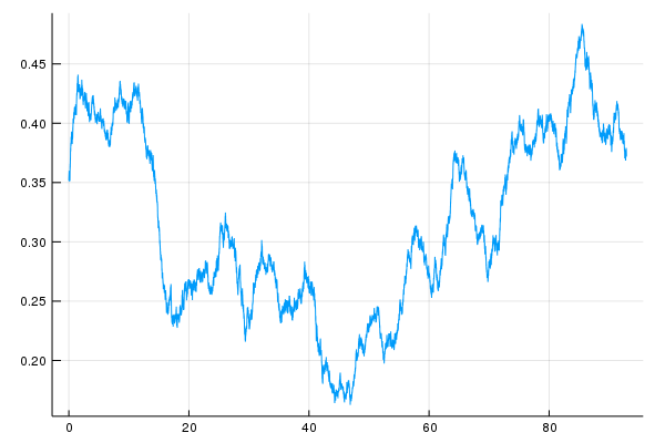
For this study, we use the SPX series from the CRSP database which is available for free to the NYU community as part of the WRDS collection of databases. In particular, we use the field that CRSP calls "Value-Weighted Return (includes distributions)". This is typically referred to as the total return. The total return is different than the returns directly from the index because of corporate actions. For example, if one of the stocks in the index provides a dividend to shareholders, that stock's price will fall the next day when it trades ex-dividend and the index will go down. However, an investor has been delivered value. The total return incorporates dividends as if the investor reinvested dividends into the index and similarly for other corporate actions such as mergers, splits and spin-offs.
The CRSP SPX series goes back to 1926, much further than the SPY ETF used in the previous study. We first reconstruct the study on this data set. Below are the approximate transition probabilities corresponding to the tertiles of this data set: \begin{eqnarray*} P \approx \left(\begin{array}{ccc} 0.39 & 0.28 & 0.33\\ 0.32 & 0.38 & 0.30\\ 0.30 & 0.34 & 0.36\\ \end{array}\right) \end{eqnarray*} Notice that, one of the key phenomena that we found to be statistically significant here, namely dead cat bounce or mean reversion from the lower state, is missing from this data. In order to see why, we calculate the transition matrix from the last 25 years of data and find the following matrix: \begin{eqnarray*} P \approx \left(\begin{array}{ccc} 0.34 & 0.25 & 0.41\\ 0.32 & 0.37 & 0.31\\ 0.34 & 0.34 & 0.32\\ \end{array}\right) \end{eqnarray*} This matrix is similar to the earlier study. So, it seems the transition probabilities change over time. Below is the chart of estimated transition from "down" to "up" using $4$ years of data which corresponds to a standard error of about $2.6\%$.
We had found this transition to be about $40\%$ in the earlier study. Notice that, in the past $25$ years, this transition rate seems to have been at this level or above. However, historically, it has been as low as $20\%$, a level that is likely to be significant in the other direction. We restrict our study to the past $25$ years. A better approach would be to model the changing transition probabilities.
We will consider investing in either cash, which we assume yields no return (since we will be investing short-term and short-term rates are typically low), or SPX. We will allow leverage up to $10$ times, that is, the strategy can invest to make between $10$ times and $-10$ times the return on SPX. Note that with equities, brokers will usually allow roughly $7$ times leverage and that only for balanced portfolios (portfolios which don't move when the market moves). In our case, our portfolio is not balanced: we are choosing to go long or short a broad market index. However, higher leverage can be achieved with futures. While futures are highly correlated with the underlier, there are some subtleties around the maturity and roll of futures contracts which we ignore for this study.
Given a set of returns $r_1, r_2, \ldots, r_k$, and a set of probabilities of those returns $p_1, p_2, \ldots, p_k$, we wish to find an optimal weight for an asset whose returns are chosen uniformly from those returns. Note that we are assuming that $r_i$ are (arithmetic) returns and log returns. Let $R$ be a random variable chosen from $r_1, r_2, \ldots, r_k$ according to the probabilities $p_1, p_2, \ldots, p_k$: \begin{eqnarray} \max_w E\left[\log\left(w(1+R) + 1-w\right)\right] & = & \max_w E\left[\log\left(wR + 1\right)\right]\\ & = & \max_w \sum_{i=1}^k p_i \log\left(w r_i + 1\right) \end{eqnarray} We take the derivative of this with respect to $w$ and set it to $0$: \begin{eqnarray} \frac{\partial}{\partial w} \sum_{i=1}^k p_i\log\left(w r_i + 1\right) & = & \sum_{i=1}^k \frac{p_i r_i}{w r_i + 1} = 0 \end{eqnarray} Note that this equation could be made into a kth order polynomial by multiplying by the denominators in the sum. However, the optimization is concave which can be seen by taking the 2nd derivative: \begin{eqnarray} \frac{\partial^2}{\partial w^2} \sum_{i=1}^k p_i\log\left(w r_i + 1\right) & = & \frac{\partial}{\partial w} \sum_{i=1}^k \frac{p_i r_i}{w r_i + 1}\\ & = & - \sum_{i=1}^k \frac{p_i r_i^2}{\left(w r_i + 1\right)^2}\\ \end{eqnarray} Note that this is strictly negative and so the objective function is strictly concave. Strictly concave optimization problems have unique solutions and can be solved numerically using nonlinear programming algorithms. Note that all of the utility functions we've discussed in this section yield concave optimization problems.
In-sample results
The following chart shows the growth over time using an optimal Kelly strategy for a 0th and 1st order model where the data is chosen in sample.
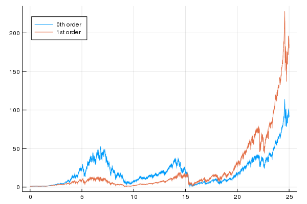
A few comments on this chart:
- The 0th order model multiplies the investor's wealth by about $100$ over 25 years and the 1st order model multiplies the investor's wealth by about $200$.
- One can see significant spikes downward. For example, the 1st order model goes from over $200$ to under $150$ in the recent past, about a $1/3$ decline though we end on an up note
- Because of the large multiples over time, it is difficult to see what happens in the earlier periods.
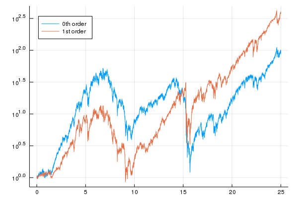
Here are some further comments on this chart:
- From this chart, it can be seem that there are very significant declines. At about year $15$, the 0th order model goes from about $10^{1.5} \approx 30$ to a bit more than $10^0 = 1$, about a $95\%$ decline. The 1st order model has about a $90\%$ decline at about the same time. These are referred to as drawdowns and are not looked upon favorably by investors.
- Furthermore, both models can take a long time to return to their previous peaks. The 0th order model has a peak at about $7$ years at a level which it doesn't return to until about $23$ years, making it about a $16$ year drawdown. The 1st order model also has a peak at about $7$ years at a level which it returns to at about $13$ years, about a $6$ year drawdown.
- Some academics have recently been investigating ways of optimizing a utility function while minimizing drawdowns but, to my knowledge, there are not many computationally tractable approaches to this problem.
- Note that we should really add additional assets to improve upon these results. For example, additional assets would allow the optimal strategy to hedge.
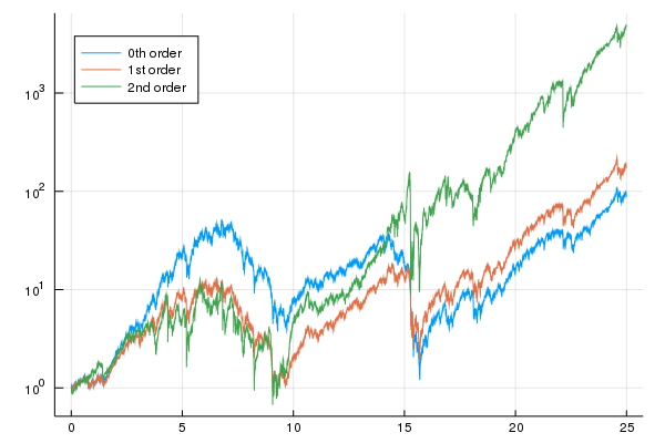
This model multiplies the investor's wealth by about 5,000. It also has much shorter drawdowns. However, it does still have drawdowns which are about an order of magnitude over $90\%$.
Out-of-sample results
In the last subsection, we demonstrated that using in sample data, that is, data taken from the same period that we were trading in, investors can do well using Markovian models even with a single asset. However, in real trading, one can only use data from the past. That means that the model and optimal weight must be chosen based only on data from the past, referred to as out of sample. In this subsection, we investigate what happens when we use out of sample data.
In order to use a model built out of sample, we'd need to recalculate the model and optimal weights for every trading period (in this case, every day) of our backtest. This would involve thousands of calculatations, each of which would involve a numerical optimization. In order to reduce the work, we calculate a new model and new weight every year. We will use data up through some year to calculate new weights, use those weights in simulated trading for the following year and iterate. Some people refer to this approach as walk forward.
We need to decide how much history to use to calculate the weights. The behavior of financial instruments tends to change over time due to changes in trader behavior, regulation, etc. Hence, choosing how much history is a balance between:
- Choosing enough history to estimate the distribution of returns well.
- Choosing enough history to capture any periodicities such as the business cycle which tends to be about $10$ years.
- Choosing little enough history so that the distribution of returns doesn't change too much.

Notice that, the results which use less than $10$ years of historical data to estimate the model, multiply the investor's money by about 1,000 times in the first $5$ years. However, they generally lose money from that point on. The backtest that uses $25$ years of historical data, generally makes a small amount of money and multiplies the investor's wealth by about $5$ in the last $5$ years of the study.
Finally, we show the same chart for the 1st order model which shows similar perforamnce.
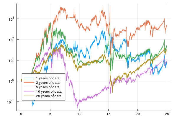
Note that only using history of $10$ years or so is enough to include large negative returns, "crashes", which keep the strategy from taking too much risk. Recall that the down-up transition reached $40\%$ about $25$ years ago. For the out of sample strategy using $10$ years of history, this would fill the history from about year $10$ in the chart. This strategy performs well from the $10$ point as shown in the chart below:
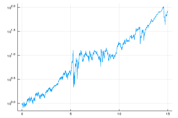
This strategy multiplies the investor's wealth by about $100$ over $15$ years with brief drawdowns of over $90\%$. The strategy does have a flat period of about $5$ years.
Optimal Trading Strategies for Hidden Markov Models
We now investigate the calculation of optimal strategies for hidden Markov models. Unlike the case of Markov chains, the current state is not observable. At any point in time, we have a distribution of possible states given the observations thus far. We can look at this distribution of possible current states as the state of the hidden Markov model.
We consider the same setup discussed previously except that the state sequence, $X_1, X_2, \ldots, X_T$ is no longer considered observable. Hence, we no longer condition on the state sequence but now only on the observed returns. As before, we are able to factor out $U\left(V_t\right)$ which facilitate the optimization, that is: \begin{eqnarray} \max_w E\left[\left.U\left(V_T\right)\right| Y_1, Y_2, \ldots, Y_t\right] & = & \max_w E\left[\left.U\left(V_tV_{t,T}\right)\right| Y_1, Y_2, \ldots, Y_t\right]\\ & = & \max_w E\left[\left.U\left(V_t\right)U\left(V_{t,T}\right)\right| Y_1, Y_2, \ldots, Y_t\right]\\ & = & \max_w U\left(V_t\right)E\left[\left.U\left(V_{t,T}\right)\right| Y_1, Y_2, \ldots, Y_t\right]\\ & = & U\left(V_t\right)\max_w E\left[\left.U\left(V_{t,T}\right)\right| Y_1, Y_2, \ldots, Y_t\right]\\ \end{eqnarray} Hence, we wish to optimize $E\left[\left.U\left(V_{t,T}\right)\right|Y_1, Y_2,\ldots, Y_t\right]$ for each $t$.
Let us consider a probability distribution, which we call $\rho$, over states. We define ${\cal V}_t^*(\rho)$ as the optimal utility from time $t$ onwards given that the distribution of states at time $t$ is $\rho$, that is: \begin{eqnarray} {\cal V}^*_t(\rho) = \max_w \sum_{i=1}^m \rho_i E\left[\left.U\left(V_{t,T}\right)\right|X_t = s_i\right] \end{eqnarray} We ultimately wish to find: \begin{eqnarray} {\cal V}_t^*\left(P\left(\left.X_t\right|Y_1,Y_2,\ldots,Y_t\right)\right) & = & \max_w \sum_{i=1}^m P\left(\left.X_t=s_i\right|Y_1,Y_2,\ldots,Y_t\right) E\left[\left.U\left(V_{t,T}\right)\right|X_t = s_i\right]\\ & = & \max_w E\left[\left.U\left(V_{t,T}\right)\right|Y_1,Y_2,\ldots,Y_t\right]\\ \end{eqnarray} We can write a recursive relationship for this quantity: \begin{eqnarray} {\cal V}_t^*\left(P\left(\left.X_t\right|Y_1,Y_2,\ldots,Y_t\right)\right) & = & \max_w E\left[\left.U\left(V_{t,T}\right)\right|Y_1,Y_2,\ldots,Y_t\right]\\ & = & \max_w E\left[\left.U\left(V_{t,t+1}V_{t+1,T}\right)\right|Y_1,Y_2,\ldots,Y_t\right]\\ & = & \max_w E\left[\left.U\left(V_{t,t+1}\right)U\left(V_{t+1,T}\right)\right|Y_1,Y_2,\ldots,Y_t\right]\\ & = & \max_w E\left[\left.E\left[\left.U\left(V_{t,t+1}\right)U\left(V_{t+1,T}\right)\right|Y_1,Y_2,\ldots,Y_t,Y_{t+1}\right]\right|Y_1,Y_2,\ldots,Y_t\right]\\ & = & \max_w E\left[\left.U\left(V_{t,t+1}\right)E\left[\left.U\left(V_{t+1,T}\right)\right|Y_1,Y_2,\ldots,Y_t,Y_{t+1}\right]\right|Y_1,Y_2,\ldots,Y_t\right]\\ & = & \max_{w_t}\max_{w_{t+1:T}} E\left[\left.U\left(V_{t,t+1}\right)E\left[\left.U\left(V_{t+1,T}\right)\right|Y_1,Y_2,\ldots,Y_t,Y_{t+1}\right]\right|Y_1,Y_2,\ldots,Y_t\right]\\ & = & \max_{w_t} E\left[\left.U\left(V_{t,t+1}\right)\max_{w_{t+1:T}} E\left[\left.U\left(V_{t+1,T}\right)\right|Y_1,Y_2,\ldots,Y_t,Y_{t+1}\right]\right|Y_1,Y_2,\ldots,Y_t\right]\\ & = & \max_{w_t} E\left[\left.U\left(V_{t,t+1}\right){\cal V}_{t+1}^*\left(P\left(\left.X_{t+1}\right|Y_1,Y_2,\ldots,Y_t,Y_{t+1}\right)\right)\right|Y_1,Y_2,\ldots,Y_t\right]\\ \end{eqnarray} This is a functional relationship between the functions ${\cal V}_t^*$ for different $t$ and involves a nonlinear optimization at each step. These equations are difficult to solve. To the authors knowledge, there are no known tractable approaches for calculating optimal trading strategies for hidden Markov models except when the utility function is Kelly.
References
-
A good reference to utility functions and terminal wealth problems is:
Bauerle, Nicole and Rieder, Ulrich. Markov Decision Processes with Applications to Finance. Springer, 2011.
-
Other approaches to solving this kind of problem are found in the field of reinforcement learning which has garnered considerable attention recently. A concise reference to this field is:
Szepesvari, Csaba. Algorithms for Reinforcement Learning. Morgan & Claypool, 2010.