Warning: MathJax requires JavaScript to process the mathematics on this page.
If your browser supports JavaScript, be sure it is enabled.

Fitting Markov chains

Maximum Likelihood Estimation

We have seen several examples of how one might analyze a Markov chain if one knows that a process is Markovian and knows the initial distribution and transition probabilities of the chain. We would now like to explore what one might do to determine the initial distribution and transition probabilities of the Markov chain.

We discuss a particular method of fitting statistical models in general, including Markov chains. To set up the problem, suppose we have a vector of $n$ observations from a statistical model, which we denote by $x^n = (x_1 x_2 \ldots x_n)$. We also suppose that there is a vector of parameters, $\theta$ of the distribution of the vector which we would like to determine. We will denote the density (or point mass function when appropriate) of the vector $x^n$ as $f_\theta{\left(x^n\right)}$.

The problem of determining the parameters is referred to as point estimation. There are several general methodologies for the problem, including maximum likelihood estimation, Bayesian estimation, statistical decision theory, the method of moments, etc. We present maximum likelihood estimation for pragmatic reasons: it is often easy and often converges to the correct answer. Other approaches can be as useful if not more so in various circumstances. We will present Bayesian estimation later in the course.

The maximum likelihood estimator, denoted by $\hat{\theta}$, of $\theta$ is the value of the $\theta$ that maximizes $f_\theta{\left(x^n\right)}$. Since the $\log$ is a monotonic function, maximizing $f_\theta{\left(x^n\right)}$ is the same as maximizing $\log f_\theta{\left(x^n\right)}$. Furthermore, if $x^n$ are independent and identically distributed (IID): \begin{eqnarray*} \log f_\theta{\left(x^n\right)} & = & \log \prod_{i=1}^n f_\theta{\left(x_i\right)} = \sum_{i=1}^n \log f_\theta{\left(x_i\right)} \end{eqnarray*} and so, maximizing the latter is often easier and is equivalent. We call the $\log$ of the density or point mass function the log likelihood function. While the log likelihood function collapses into a sum of log densities in the IID case, we present maximum likelihood estimation in the more general context since we are ultimately interested in maximum likelihood estimation for Markov chains which are not IID.

Example: Normal Mean and Variance

We give an example of maximum likelihood estimation in the case of estimating the mean and variance of a normal distribution. Let $X_1, X_2, \ldots$ be IID random variables with distribution $N(\mu,\sigma^2)$ where both $\mu$ and $\sigma$ are unknown parameters. The parameter vector is given by: \begin{eqnarray} \theta = \left(\begin{array}{c}\mu\\ \sigma\end{array}\right) \end{eqnarray} Given observations $x^n = (x_1 x_2 \ldots x_n)$, the log likelihood function is given by: \begin{eqnarray*} \log f_\theta{\left(x^n\right)} & = & \log \prod_{i=1}^n \frac{1}{\sqrt{2 \pi \sigma^2}} \exp{\left(-\frac{\left(x_i - \mu\right)^2}{2\sigma^2}\right)}\\ & = & \sum_{i=1}^n \left(-\log{\sqrt{2 \pi \sigma^2}} - \frac{\left(x_i - \mu\right)^2}{2\sigma^2}\right)\\ & = & -\frac{n}{2} \log{\left(2 \pi \sigma^2\right)} - \sum_{i=1}^n \frac{\left(x_i - \mu\right)^2}{2\sigma^2}\\ \end{eqnarray*} Differentiating with respect to $\mu$ and equating to $0$ yields: \begin{eqnarray*} \frac{\partial}{\partial \mu} \log f_\theta{\left(x^n\right)} & = & \frac{\partial}{\partial \mu}\left(-\frac{n}{2} \log{\left(2 \pi \sigma^2\right)} - \sum_{i=1}^n \frac{\left(x_i - \mu\right)^2}{2\sigma^2}\right)\\ & = & \sum_{i=1}^n \frac{x_i - \mu}{\sigma^2} = 0 \end{eqnarray*} which, after rearranging becomes: \[ \hat{\mu} = \frac{1}{n}\sum_{i=1}^n x_i \] where we have used the notation $\hat{\mu}$ to signify that this is the maximum likelihood estimator. Now differentiating with respect to $\sigma$ and setting to $0$ yields: \begin{eqnarray*} \frac{\partial}{\partial \sigma} \log f_\theta{\left(x^n\right)} & = & \frac{\partial}{\partial \sigma}\left(-\frac{n}{2} \log{\left(2 \pi \sigma^2\right)} - \sum_{i=1}^n \frac{\left(x_i - \mu\right)^2}{2\sigma^2}\right)\\ & = & -\frac{n}{\sigma} + \sum_{i=1}^n \frac{\left(x_i - \hat{\mu}\right)^2}{\sigma^3} = 0 \end{eqnarray*} where we have substituted in the solution for $\mu$, namely, $\hat{\mu}$. Multiplying by $\sigma$ and rearranging yields: \[ \hat{\sigma} = \sqrt{\frac{\sum_{i=1}^n \left(x_i - \hat{\mu}\right)^2}{n}} \] Hence, the maximum likelihood estimator of a normal mean and variance are the sample mean and variance. Note that this formula is sometimes called the "biased sample variance" since it is biased (though asymptotically unbiased). If the $\frac{1}{n}$ factor is replaced by $\frac{1}{n-1}$, it becomes unbiased but is no longer the maximum likelihood estimator. The biased and unbiased sample variances behave very similarly asymptotically.

Example: Lognormal Mean and Variance

Now let $Y_1, Y_2, \ldots$ be IID with a lognormal distribution with parameters $\mu$ and $\sigma$. Note that $Y_i = \exp{\left(X_i\right)}$ where $X_1, X_2, \ldots$ are IID normal with mean $\mu$ and variance $\sigma^2$. The maximum likelihood estimator of the parameters of a sequence of transformed random variables is the maximum likelihood estimator of the original random variables, that is, after applying the inverse transformation to the transformed random variables. Hence: \begin{eqnarray*} \hat{\mu} = \frac{1}{n}\sum_{i=1}^n \log{\left(x_i\right)}\\ \hat{\sigma} = \sqrt{\frac{\sum_{i=1}^n\left(\log{\left(x_i\right)} - \hat{\mu}\right)^2}{n}}\\ \end{eqnarray*} The maximum likelihood estimator of the parameters of lognormal random variables is the sample mean and standard deviation of the $\log$ of the random variables.

Example: The Binomial Distribution

We now give an example of maximum likelihood estimation in the case of a binomial distribution, as the term is used in statistics. Note that this model is slightly different from the binomial tree model in derivative pricing. Let $X_1, X_2, \ldots$ be a sequence of IID random variables such that: \[ X_i = \left\{\begin{array}{rl}0 & \mbox{w.p. $1-p$}\\ 1 & \mbox{w.p. $p$}\\\end{array}\right. \] for some parameter $p\in[0,1]$. The log likelihood function of some observations $x_1, x_2, \ldots$ is given by: \begin{eqnarray*} \log f_p{\left(x^n\right)} & = & \log \prod_{i=1}^n p^{x_i} (1-p)^{1-x_i} = \sum_{i=1}^n \left(x_i \log p + \left(1-x_i\right) \log \left(1-p\right)\right)\\ & = & n_1{\left(x^n\right)} \log p + n_0{\left(x^n\right)} \log \left(1-p\right) \end{eqnarray*} where $n_y{\left(x^n\right)}$ denotes the number of occurences of $y$ in $x^n$. We find a maximum of this with respect to $p$ by setting its derivative with respect to $p$ to $0$: \begin{eqnarray*} \frac{\partial}{\partial p}\log f_p{\left(x^n\right)} & = & \frac{\partial}{\partial p}n_1{\left(x^n\right)} \log p + n_0{\left(x^n\right)} \log \left(1-p\right)\\ & = & \frac{n_1{\left(x^n\right)}}{p} - \frac{n_0{\left(x^n\right)}}{1-p} = 0 \end{eqnarray*} Multiplying by $p$ and $1-p$ yields: \[ n_1{\left(x^n\right)}\left(1-p\right) - n_0{\left(x^n\right)}p = 0 \] which produces: \[ \hat{p} = \frac{n_1{\left(x^n\right)}}{n_1{\left(x^n\right)} + n_0{\left(x^n\right)}} = \frac{n_1{\left(x^n\right)}}{n} \] where we have used the fact that $n_1{\left(x^n\right)} + n_0{\left(x^n\right)} = n$. Hence, the maximum likelihood estimate of the probability of an IID binomial model is the frequency of occurence of $1$. Note that we have use $\hat{p}$ in the last equation to emphasize that this is the maximum likelihood estimator.

Example: The Multinomial Model

We now generalize the previous example to the case when there are more than $2$ possible outcomes (in the previous example, we used $0$ and $1$ as the possible outcomes). Let $X_1, X_2, \ldots$ be IID random variables with values in the set $\left\{s_1, s_2, \ldots, s_m\right\}$ with corresponding probabilities $p = \left(p_1 p_2 \ldots p_m\right)$. The log likelihood function of the observations $x^n$ is given by: \begin{eqnarray*} \log f_p{\left(x^n\right)} & = & \log \prod_{i=1}^n p_{x_i} = \log \prod_{i=1}^n \prod_{j=1}^m p_j^{n_{s_j}{\left(x_i\right)}} = \sum_{i=1}^n \sum_{j=1}^m n_{s_j}{\left(x_i\right)}\log p_j\\ & = & \sum_{j=1}^m \sum_{i=1}^n n_{s_j}{\left(x_i\right)}\log p_j = \sum_{j=1}^m n_{s_j}{\left(x^n\right)}\log p_j \end{eqnarray*} Note that we must have $\sum_{i=1}^m p_i = 1$ so we will add a Lagrange multiplier, $\lambda$ for this constraint, and equate the derivative with respect to $p_k$ to $0$: \begin{eqnarray*} \frac{\partial}{\partial p_k} \log f_p{\left(x^n\right)} & = & \frac{\partial}{\partial p_k}\left(\sum_{j=1}^m n_{s_j}{\left(x^n\right)}\log p_j - \lambda\left(\sum_{j=1}^m p_j-1\right)\right)\\ & = & \frac{n_{s_k}{\left(x^n\right)}}{p_k} - \lambda = 0 \end{eqnarray*} so that we have: \[ p_k = \frac{n_{s_k}{\left(x^n\right)}}{\lambda} \] The equation $\sum_{j=1}^m p_j = 1$ now becomes: \[ \sum_{j=1}^m \frac{n_{s_j}{\left(x^n\right)}}{\lambda} = 1 \] which implies that: \[ \lambda = \sum_{j=1}^m n_{s_j}{\left(x^n\right)} = n \] so that: \[ \hat{p}_k = \frac{n_{s_k}{\left(x^n\right)}}{n} \] Again here, the maximum likelihood estimate of the probability that $s_k$ occurs is the frequency of occurence of $s_k$ in the sample.

Example: Markov Chain Transition Probabilities

We now suppose we observe the state sequence of a finite homogeneous Markov chain. For the moment, we will assume that we know the initial probabilities and would like to determine the transition probabilities. Let the states of the Markov chain be $\left\{s_1,\ldots,s_m\right\}$. We let the initial probabilities be $\pi$ and the transition probabilities $p_{s_i,s_j}$. The log likelihood function of observations $x^n$ is given by: \begin{eqnarray*} \log f_P{\left(x^n\right)} & = & \log\left( \pi_{x_1} \prod_{i=2}^n p_{x_{i-1},x_i}\right) = \log \left(\pi_{x_1} \prod_{i=2}^n \prod_{j=1}^m \prod_{k=1}^m p_{s_j,s_k}^{n_{s_j,s_k}{\left(x_{i-1} x_i\right)}}\right) = \log \pi_{x_1} + \sum_{i=2}^n \sum_{j=1}^m \sum_{k=1}^m n_{s_j,s_k}{\left(x_{i-1} x_i\right)}\log p_{s_j,s_k}\\ & = & \log \pi_{x_1} + \sum_{j=1}^m \sum_{k=1}^m \sum_{i=2}^n n_{s_j,s_k}{\left(x_{i-1} x_i\right)}\log p_{s_j,s_k} = \log \pi_{x_1} + \sum_{j=1}^m \sum_{k=1}^m n_{s_j,s_k}{\left(x^n\right)}\log p_{s_j,s_k}\\ \end{eqnarray*} where $n_{s_j,s_k}{\left(x_{i-1}x_i\right)}$ is the number of occurences of $s_j$ followed by $s_k$ in the sequence $x_{i-1} x_i$ (which, in this case is either $0$ or $1$) and $n_{s_j,s_k}{\left(x^n\right)}$ is the number of occurences of $s_j$ followed by $s_k$ in the sequence $x^n$. Note that we have the $m$ constraints that each row of the transition probability matrix sums to $1$, that is, $\sum_{k=1}^m p_{s_j,s_k} = 1$ for any $j\in\left\{1,\ldots,m\right\}$. We add a Lagrange multiplier $\lambda_j$ corresponding to each of these constraints and set the derivative with respect to $p_{s_{j'},s_{k'}}$ to $0$: \begin{eqnarray*} \frac{\partial}{\partial p_{s_{j'},s_{k'}}} \log f_P{\left(x^n\right)} & = & \frac{\partial}{\partial p_{s_{j'},s_{k'}}}\left(\log \pi_{x_1} + \sum_{j=1}^m \sum_{k=1}^m n_{s_j,s_k}{\left(x^n\right)}\log p_{s_j,s_k} - \sum_{j=1}^m \lambda_j \left(\sum_{k=1}^m p_{s_j,s_k}-1\right)\right)\\ & = & \frac{n_{s_{j'},s_{k'}}{\left(x^n\right)}}{p_{s_{j'},s_{k'}}} - \lambda_{j'} = 0\\ \end{eqnarray*} so that we have: \[ p_{s_{j'},s_{k'}} = \frac{n_{s_{j'},s_{k'}}{\left(x^n\right)}}{\lambda_{j'}} \] The equation $\sum_{k=1}^m p_{s_j,s_k} = 1$ now becomes: \[ \sum_{k=1}^m \frac{n_{s_j,s_k}{\left(x^n\right)}}{\lambda_j} = 1 \] which implies that: \[ \lambda_j = \sum_{k=1}^m n_{s_j,s_k}{\left(x^n\right)} \] Note that this quantity is the number of occurences of $s_j$ in the sequence of observations $x_1, x_2, \ldots, x_{n-1}$. The final result is: \begin{eqnarray} \hat{p}_{s_j,s_k} = \frac{n_{s_j,s_k}{\left(x^n\right)}}{\sum_{k=1}^m n_{s_j,s_k}{\left(x^n\right)}}\label{eq:transitionprobability} \end{eqnarray} In words, the maximum likelihood estimate the transition probability from $s_j$ to $s_k$ is the number of times we see $s_j$ followed by $s_k$ as a fraction of the number of times we see $s_j$ followed by any other state.

Note that the transition matrix previously mentioned for credit rating migrations was fit using a formula very similar to this.

Example: Laplace Distribution

Thus far, the maximum likelihood estimators have all turned out to be the sample means and variances of the quantities being estimated. We now give an example of a maximum likelihood estimator which is not based on sample means, namely, the maximum likelihood estimator of the mean of the Laplace distribution. The Laplace distribution is given by: \begin{eqnarray*} f_\mu\left(x\right) = \frac{1}{2}\exp\left( -\left| x - \mu \right| \right) \end{eqnarray*} Note that the mean is $\mu$. This distribution has been proposed as a better model for stock prices since it has slightly heavier tails than the normal distribution. We find the maximum likelihood estimator by setting the derivative of the log likelihood equal to $0$: \begin{eqnarray*} \frac{\partial}{\partial \mu}\sum_i \left(\log\frac{1}{2} - \left| x_i - \mu\right|\right) = \sum_{i:x_i>\mu} 1 + \sum_{i:x_i<\mu} \left(-1\right) = 0 \end{eqnarray*} The above equation is satisfied if we choose $\mu$ so that the number of $x_i$ above $\mu$ is the same as the number of $x_i$ below $\mu$, that is, by the sample median.

Consistency of Maximum Likelihood for IID Sequences

In this section, we explore whether the maximum likelihood estimator is a good estimator. If maximum likelihood is a good estimator, one would expect, at a minimum, that the observations are drawn according to the distribution $f_{\theta^*}$, then $\hat{\theta}$ would converge towards $\theta^*$ as the number of observations tended to $\infty$. This property is called consistency. Consider the log likelihood function in the IID case: \[ \log f_\theta{\left(x^n\right)} = \sum_{i=1}^n \log f_\theta{\left(x_i\right)} \] Since this is a sum of IID random variables, the law of large numbers can be applied to $\frac{1}{n}$ times it. Using this result, we can find the asymptotic behavior of the log likelihood function: \begin{eqnarray*} \lim_{n\rightarrow\infty} \frac{1}{n} \sum_{i=1}^n \log f_\theta{\left(X^n\right)} = E_{\theta^*}{\left[\log f_\theta{\left(X_i\right)}\right]} \end{eqnarray*} where $E_{\theta^*}$ denotes expectation with respect to a random IID sequence drawn from the distribution $f_{\theta^*}$. The expression on the right hand side is called the cross entropy. We will now show that the cross entropy is maximized when $\theta = \theta^*$.

The maximum of $E_{\theta^*}{\left[\log f_\theta{\left(X_i\right)}\right]}$ over all $\theta$ is given by $\theta=\theta^*$.

Note that $\log$ is a concave function so $-\log$ is convex. Hence: \begin{eqnarray*} E_{\theta^*}{\left[\log f_\theta{\left(X_i\right)}\right]} & = & E_{\theta^*}{\left[\log f_\theta{\left(X_i\right)}\right]} - E_{\theta^*}{\left[\log f_{\theta^*}{\left(X_i\right)}\right]} + E_{\theta^*}{\left[\log f_{\theta^*}{\left(X_i\right)}\right]}\\ & = & E_{\theta^*}{\left[\log{\left(\frac{f_\theta{\left(X_i\right)}}{f_{\theta^*}{\left(X_i\right)}}\right)}\right]} + E_{\theta^*}{\left[\log f_{\theta^*}{\left(X_i\right)}\right]}\\ & = & -E_{\theta^*}{\left[-\log{\left(\frac{f_\theta{\left(X_i\right)}}{f_{\theta^*}{\left(X_i\right)}}\right)}\right]} + E_{\theta^*}{\left[\log f_{\theta^*}{\left(X_i\right)}\right]}\\ & \leq & \log{\left(E_{\theta^*}{\left[\frac{f_\theta{\left(X_i\right)}}{f_{\theta^*}{\left(X_i\right)}}\right]}\right)} + E_{\theta^*}{\left[\log f_{\theta^*}{\left(X_i\right)}\right]}\\ & = & \log\int\frac{f_\theta{\left(X_i\right)}}{f_{\theta^*}{\left(X_i\right)}}f_{\theta^*}{\left(X_i\right)}dX_i + E_{\theta^*}{\left[\log f_{\theta^*}{\left(X_i\right)}\right]}\\ & = & E_{\theta^*}{\left[\log f_{\theta^*}{\left(X_i\right)}\right]}\\ \end{eqnarray*} The result holds since the last expression is achieved by setting $\theta = \theta^*$ in the first expression.

Since the log likelihood function converges to the cross entropy and the cross entropy is maximized at the true parameter, it is plausible that the maximum of the log likelihood converge to the true value. There are some relatively mild technical conditions required in order to interchange maximization and expected value.

Consistency of Maximum Likelihood for Markov Chains

In the last section, we discussed how, under general conditions, the maximum likelihood estimate for an IID process is consistent, meaning that it converges to the true parameter. We now investigate this question for Markov chains where there is some more subtlety. We first give an example of one subtlety.

Example: Markov Chains with Transient States

Consider a Markov chain, such as the mortgage default model, which contains transient states. The Markov chain will spend only a finite number of steps in the transient states on any single path. If our observations consist of a single path, we will not be able to consistently estimate the transition probabilities among the transient states. For example, in the mortgage default model, it is possible for the chain to go from state $C$ directly to state $P$ on the first iteration. In this case, the estimate given in (\ref{eq:transitionprobability}) would be: \[ \hat{p}_{C,P} = 1\\ \] \[ \hat{p}_{C,C} = 0\\ \] \[ \hat{p}_{C,30} = 0\\ \] \[ \hat{p}_{30,C} = \frac{0}{0}\\ \] \[ \hat{p}_{30,30} = \frac{0}{0}\\ \] \[ \hat{p}_{30,60} = \frac{0}{0}\\ \] \[ \hat{p}_{60,C} = \frac{0}{0}\\ \] \[ \hat{p}_{60,60} = \frac{0}{0}\\ \] \[ \hat{p}_{60,D} = \frac{0}{0}\\ \] Since these are not correct even though this path happens with positive probability, the estimate is inconsistent for a single sample path. Note that, if we have multiple independent sample paths, the case is very different. As the number of sample paths grow, we can estimate the transition probabilities without issue. In this case, the consistency proof of the IID case holds. This is the case which occurs in mortgage modeling: in industry, these models are often fit with the sample paths from millions of loans.

Since, as discussed in the previous example, maximum likelihood with observations which consist of many sample paths is equivalent to IID observations where maximum likelihood is known to be consistent under general conditions, we focus instead on a single, long sample path. This is the case of the regime-switching models, where the observations consisted of a single 4,347 length path. For this case, we present the following theorem, which is a law of large numbers for Markov chains:

For any irreducible Markov chain, equation (\ref{eq:transitionprobability}) converges to the transition probabilities.

Higher Order Markov Chains

While the next state of a Markov chains is dependent only upon its current state, it is possible that a random process has dependencies that go back several states in the past. A sequence of random variables $X_1, X_2, \ldots$ is an $k$th order Markov chain if for any $t>n$ and states $s_1, s_2, \ldots s_{t+1}$: \[ \mathbb{P}\left(X_t=s_t\right|\left.X_1 = s_1, X_2=s_2, \ldots, X_{t-1}=s_{t-1}\right) = \mathbb{P}\left(X_t=s_t\right|\left. X_{t-k}=s_{t-k}, X_{t-k+1}=s_{t-k+1}, \ldots, X_{t-1}=s_{t-1}\right) \] Note that a first order Markov chain is the Markov chain that we have been studying thus far. A second order Markov chain is a process whose next state is dependent upon the current and previous state.

A $k$th order Markov chain can be represented as a first order Markov chain on a larger state space, specifically, on the state space of the $k$ most recent observations. We demonstrate this for $k=2$. Let $X_1, X_2, \ldots$ be a second order Markov chain. Consider the process consisting of the pair of the current and most recent past random variables, $\left(X_{t-1}, X_t\right)$. Note that $X_{t-1}$ is completely determined by $\left(X_{t-2},X_{t-1}\right)$ and, since the process is a second order Markov chain, $X_t$ is independent of $X_1, \ldots, X_{t-3}$ given $\left(X_{t-2},X_{t-1}\right)$. \begin{eqnarray*} \mathbb{P}\left(\left(X_{t-1},X_t\right)=\left(s_{t-1},x_t\right) \right|\left.\left(X_1,X_2\right) = \left(s_1, s_2\right), \left(X_2,X_3\right)=\left(s_2,s_3\right), \ldots, \left(X_{t-2},X_{t-1}\right)=\left(s_{t-2},s_{t-1}\right)\right)\\ = \mathbb{P}\left(\left(X_{t-1},X_t\right)=\left(s_{t-1},x_t\right) \right|\left.\left(X_{t-2},X_{t-1}\right)=\left(s_{t-2},s_{t-1}\right)\right)\\ \end{eqnarray*} So that the vector-valued process, $\left(X_1,X_2\right), \left(X_2,X_3\right), \ldots$ is a (first order) Markov chain.

Example: Second Order Chain

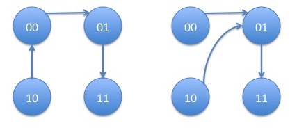
In this example we discuss a second order Markov chain on the binary state space $\{0,1\}$. We will write $p_{s_1s_2,s_3}$ for the transition probability to $s_3$ given $s_1$ and $s_2$ were the two most recent states. As in the last paragraph, we consider the vector of pairs of states to make this process into a first order process on a larger state space. The graph of this Markov chain is:

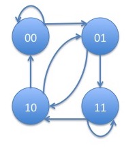
From the state pair $00$, we can go either to $00$ (itself) or $01$. From the state pair $01$, we can go either to $10$ or $11$. From the state pair $10$, we can go either to $00$ or $01$. From the state pair $11$, we can go either to $10$ or $11$ (itself). Note that, if all the possible transition probabilities are positive, the chain is irreducible since every state can reach every other state. It is also aperiodic since it has self-loops which are cycles of length $1$ and the greatest common divisor of any set of numbers containing $1$ is $1$. Hence, the Perron-Frobenius theorem holds and the Markov chain would converge geometrically to its stationary distribution.

We now determine the formula for the stationary distribution of the Markov chain using the Markov chain tree theorem. The trees tending to state pair $00$ are:

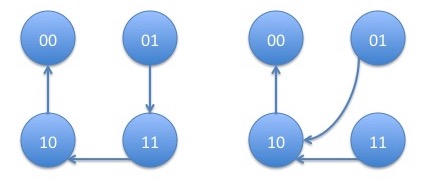
with corresponding products: \begin{eqnarray*} p_{01,1}p_{10,0}p_{11,0} + p_{01,0}p_{10,0}p_{11,0} = p_{10,0}p_{11,0} \end{eqnarray*} The trees tending to state pair $01$ are:

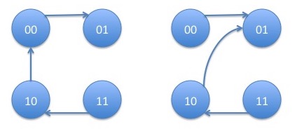
with corresponding products: \begin{eqnarray*} p_{00,1}p_{10,0}p_{11,0} + p_{00,1}p_{10,1}p_{11,0} = p_{00,1}p_{11,0} \end{eqnarray*} The trees tending to state pair $10$ are:

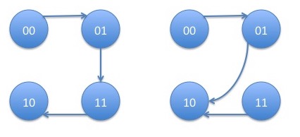
with corresponding products: \begin{eqnarray*} p_{00,1}p_{01,1}p_{11,0} + p_{00,1}p_{01,0}p_{11,0} = p_{00,1}p_{11,0} \end{eqnarray*} The trees tending to state pair $11$ are:

with corresponding products: \begin{eqnarray*} p_{00,1}p_{01,1}p_{10,0} + p_{00,1}p_{01,1}p_{10,1} = p_{00,1}p_{01,1} \end{eqnarray*} Hence, the stationary distribution is given by: \begin{eqnarray}\label{eq:stationary} \left(\begin{array}{c} \pi_{00}\\ \pi_{01}\\ \pi_{10}\\ \pi_{11}\\ \end{array}\right) = c \left(\begin{array}{c} p_{10,0}p_{11,0}\\ p_{00,1}p_{11,0}\\ p_{00,1}p_{11,0}\\ p_{00,1}p_{01,1}\\ \end{array}\right) \end{eqnarray} where: \begin{eqnarray*} c = \frac{1}{p_{10,0}p_{11,0} + p_{00,1}p_{11,0} + p_{00,1}p_{11,0} + p_{00,1}p_{01,1}} \end{eqnarray*} Note that, in particular, we always have that $\pi_{01} = \pi_{10}$. This example shows that every second order Markov chain on $2$ states can be represented as a first order Markov chain on $4$ states. However, the converse is not true: not every first Markov chain on $4$ states is a second order Markov chain on $2$ states since some of the transitions don't occur in the graph.

IID processes are sometimes called memoryless processes. Markov chains allow us to model dependence in random variables, or memory. Higher order Markov chains allow us to model higher-order dependence in random variables. However, there are stochastic processes which are not Markov of any order. One such process are regime-switching models. Note that while the underlying hidden regime is Markovian, the observed market returns are not. We will discuss this further when we talk about these models in detail. For example, recall that in the $2$-state regime-switching model, the market moves $-0.10\% \pm 1.96\%$ in the first state and $0.07\%\pm 0.72\%$ in the second state. If we see an observation which is $\le -0.10\%$ then it presents evidence that we are in the first state but it is not definitive: the observation would happen with $50\%$ probability from the first state and $41\%$ probability from the second state. If we we were to see two observations which are $\le -0.10\%$ then it presents further evidence that we are in the first state but it is still not definitive: these observations happen with $25\%$ probability from the first state while only $17\%$ probability from the second state. The greater number of negative observations, we have, the more evidence that we are in the first state but we will never be certain. While not every stochastic process is Markov of some order, it is important to note that any discrete stochastic process can be approximated arbitrarily well by a sufficiently high order Markov chain.

Maximum Likelihood Estimator for Higher Order Markov Chains

We find the maximum likelihood estimator for a higher order Markov chain using the representation as a Markov chain on a larger state space. As mentioned previously, the maximum likelihood estimator of some transformed data is the maximum likelihood estimator of the original data with the inverse transformation applied. The pairing of the states is just such a transformation. We demonstrate the result for a second order Markov chain. The generalization to $k$th order Markov chains is straightforward.

Given data, $x^n$, from a second order Markov chain, by pairing the states and using equation (\ref{eq:transitionprobability}), we have: \begin{eqnarray*} \hat{p}_{\left(s_i,s_j\right),\left(s_k,s_l\right)} = \frac{n_{\left(s_i,s_j\right),\left(s_k,s_l\right)}{\left(x^n\right)}}{\sum_{k=1}^m\sum_{l=1}^m n_{\left(s_i,s_j\right),\left(s_k,s_l\right)}{\left(x^n\right)}} \end{eqnarray*} Note that the second element of the first pair has to equal the first element of the subsequent pair, since those pairs represent $\left(X_{t-1},X_t\right)$ and $\left(X_t,X_{t+1}\right)$, respectively. Hence, $s_j=s_k$ in the above equation. Applying the inverse transformation the equation becomes: \begin{eqnarray*} \hat{p}_{s_is_j,s_l} = \frac{n_{s_i,s_j,s_l}{\left(x^n\right)}}{\sum_{l=1}^m n_{s_i,s_j,s_l}{\left(x^n\right)}} \end{eqnarray*}

Model Order Selection and Hypothesis Testing

In most practical situations, and all practical situations that I know of in finance, there is no "right" model. Finance involves the behavior of people, and while there may be statistical regularity in people's behavior, the actual behavior of individuals is impossible to predict with a finite model. It is my belief that there is a series of more and more complex models which can more and more accurately reflect reality. However, as one fits a model with more and more parameters, the mean squared error of the estimates of the parameters from the actual parameters goes up. As an example of an extreme case, if we were to fit a $n$th order Markov chain from an $n$ length sequence of data, we can fit perfectly: the likelihood of the data given the model would be $100\%$. However, we would be "overfitting" (often called data mining or curve fitting these days) and the mean squared error of the estimates of the transition probability to the actual transition probabilities would be very far apart. Overfitting is an extremely common phenomenon in finance. Determining how to find the correct model is the part of the art of statistics and machine learning: there are many approaches and no consensus has emerged. Here, we present one approach which works at least for some models: the log likelihood ratio test.

Consider a statistical problem where we have two possible parameter sets $\Theta_0$ and $\Theta_1$. We wish to determine which of the sets the true parameters $\theta^*$ is contained in. The statistical problem of determining whether the true parameter falls in $\Theta_0$ or $\Theta_1$ is called hypothesis testing. Hypothesis testing proceeds by measuring some property of the data, called a test statistic, which we denote by $T\left(x^n\right)$. Note that in some cases, we might have $\Theta_0\subseteq\Theta_1$ which are referred to as nested. If this is the case, we wish to determine whether the true parameter belongs to $\Theta_0$ or $\Theta_1 - \Theta_0$. For example, $\Theta_0$ could be the set of IID stochastic processes and $\Theta_1$ the set of Markov chains. If one chooses the transition probabilities of a Markov chain such that $p_{s,u} = p_{t,u}$ for all states $s$, $t$ and $u$, then the Markov chain is IID. However, in this case, we wish to know whether the stochastic process is IID or whether it is Markovian and not IID. A similar situation occurs when deciding whether the process is best modeled by a $k$th order Markov chain or a $k+1$th order Markov chain. These will be the motivating examples of this section.

When $\Theta_0\subseteq\Theta_1$ are nested models, the log likelihood of any data set within the set $\Theta_1$ is always more than the likelihood within $\Theta_0$: \begin{eqnarray*} \sup_{\theta\in\Theta_1} \log f_\theta\left(x^n\right)\ge\sup_{\theta\in\Theta_0} \log f_\theta\left(x^n\right) \end{eqnarray*} since we can always choose an element of $\Theta_0$ as an element of $\Theta_1$. It turns out, that under certain conditions, the distribution of how much bigger asymptotically converges to the $\chi^2$ distribution:

When the true parameter, $\theta^*\in \Theta_0$ and under some other technical conditions, we have: \begin{eqnarray*} \lim_{n\rightarrow\infty} \mathbb{P}\left(2 \log \left(\frac{\max_{\theta\in\Theta_1}f_\theta\left(x^n\right)}{\max_{\theta\in\Theta_0}f_\theta\left(x^n\right)}\right)\leq \alpha\right) = F_k(\alpha) \end{eqnarray*} where $k$ is the difference in the number of dimensions between $\Theta_1$ and $\Theta_0$ and $F_k$ is the cumulative distribution function of the $\chi^2$ distribution with $k$ degrees of freedom.

This suggests using the log likelihood ratio as the test statistic: \begin{eqnarray*} T\left(x^n\right) = 2 \log \left(\frac{\max_{\theta\in\Theta_1}f_\theta\left(x^n\right)}{\max_{\theta\in\Theta_0}f_\theta\left(x^n\right)}\right) \end{eqnarray*} We can test for this hypothesis by choosing the larger hypothesis if the probability of the log likelihood ratio is sufficiently large that it would be unlikely to occur randomly when the smaller hypothesis is true.

A few notes about this test:

Since we are fitting a model over $\Theta_0$ and one over $\Theta_1$, it is important that the maximization is incorporated into the test statistic.

The power of the above theorem is that it holds for a wide variety of processes. There are many statistical tests for specific situations, such as the following test statistic: \begin{eqnarray*} T\left(x^n\right) = \frac{\left(\sum_{i=1}^m \sum_{j=1}^m n_{s_i,s_j}{\left(x^n\right)} - \frac{\sum_{i=1}^m n_{s_i,s_j}{\left(x^n\right)}\sum_{j=1}^m n_{s_i,s_j}{\left(x^n\right)}}{n}\right)^2}{\frac{\sum_{i=1}^m n_{s_i,s_j}{\left(x^n\right)}\sum_{j=1}^m n_{s_i,s_j}{\left(x^n\right)}}{n}} \end{eqnarray*} which is also asymptotically $\chi^2$ distributed. However, this test statistic only works for Markov chains and only using the full parameterization (in some cases, one might want to fit fewer parameters). The log likelihood ratio test works for a wide variety of models.

In addition, the log likelihood test is convenient. Most likely, we don't only want to distinguish between $\Theta_0$ and $\Theta_1$ but we also want to choose a particular parameter within the model we believe to be a better fit. If we are planning on doing maximum likelihood estimation, this test statistic is very convenient.

Example: a Multinomial versus Markov Test

Consider a process $X_1, X_2, \ldots$ which we believe is either multinomial IID or Markov. The log likelihood of the multinomial model can be derived by substituting the form of the maximum likelihood estimator back into the log likelihood function: \begin{eqnarray*} \max_p \log f_p{\left(x^n\right)} = \sum_{j=1}^m n_{s_j}{\left(x^n\right)} \log {\left(\frac{n_{s_j}{\left(x^n\right)}}{n}\right)} \end{eqnarray*} Similarly, the log likelihood of the Markov chain can be derived by substituting the form of the maximum likelihood estimator back into the log likelihood function: \begin{eqnarray*} \max_p \log f_p{\left(x^n\right)} = \log \pi_{s_1} + \sum_{j=1}^m\sum_{k=1}^m n_{s_j,s_k}{\left(x^n\right)} \log {\left(\frac{n_{s_j,s_k}{\left(x^n\right)}}{\sum_{k=1}^m n_{s_j,s_k}{\left(x^n\right)}}\right)} \end{eqnarray*} The log of the ratio of the likelihoods is the difference of the likelihoods so the test statistic is given by: \begin{eqnarray*} \lefteqn{2 \log \left(\frac{\max_{\theta\in\Theta_1}f_\theta\left(x^n\right)}{\max_{\theta\in\Theta_0}f_\theta\left(x^n\right)}\right)}\\ & = & 2\left(\log \pi_{s_1} + \sum_{j=1}^m\sum_{k=1}^m n_{s_j,s_k}{\left(x^n\right)} \log {\left(\frac{n_{s_j,s_k}{\left(x^n\right)}}{\sum_{k=1}^m n_{s_j,s_k}{\left(x^n\right)}}\right)} - \sum_{j=1}^m n_{s_j}{\left(x^n\right)} \log {\left(\frac{n_{s_j}{\left(x^n\right)}}{n}\right)}\right)\\ \end{eqnarray*} Note that, since the initial distribution can't be estimated, we condition on the first observation which is inconsequential asymptotically and simplifies the test statistic a bit: \begin{eqnarray*} \lefteqn{2 \log \left(\frac{\max_{\theta\in\Theta_1}f_\theta\left(x^n|x_1\right)}{\max_{\theta\in\Theta_0}f_\theta\left(x^n|x_1\right)}\right)}\\ & = & 2\left(\sum_{j=1}^m\sum_{k=1}^m n_{s_j,s_k}{\left(x^n\right)} \log {\left(\frac{n_{s_j,s_k}{\left(x^n\right)}}{\sum_{k=1}^m n_{s_j,s_k}{\left(x^n\right)}}\right)} - \sum_{j=1}^m \sum_{k=1}^m n_{s_j,s_k}{\left(x^n\right)} \log {\left(\frac{\sum_{j=1}^m n_{s_j,s_k}{\left(x^n\right)}}{\sum_{j=1}^m\sum_{k=1}^m n_{s_j,s_k}{\left(x^n\right)}}\right)}\right)\\ & = & 2\sum_{j=1}^m\sum_{k=1}^m n_{s_j,s_k}{\left(x^n\right)} \log {\left(\frac{n_{s_j,s_k}{\left(x^n\right)}\sum_{j=1}^m\sum_{k=1}^m n_{s_j,s_k}{\left(x^n\right)}}{\sum_{k=1}^m n_{s_j,s_k}{\left(x^n\right)}\sum_{j=1}^m n_{s_j,s_k}{\left(x^n\right)}}\right)}\\ \end{eqnarray*}

Example: a Markov versus Second Order Markov Test

Using a similar analysis as multinomial versus Markov, we can calculate the test statistic of Markov versus second order Markov as: \begin{eqnarray*} \lefteqn{2 \log \left(\frac{\max_{\theta\in\Theta_1}f_\theta\left(x^n|x_1,x_2\right)}{\max_{\theta\in\Theta_0}f_\theta\left(x^n|x_1,x_2\right)}\right)}\\ & = & 2\sum_{i=1}^m\sum_{j=1}^m\sum_{k=1}^m n_{s_i,s_j,s_k}{\left(x^n\right)} \log {\left(\frac{n_{s_i,s_j,s_k}{\left(x^n\right)}\sum_{i=1}^m\sum_{k=1}^m n_{s_i,s_j,s_k}{\left(x^n\right)}}{\sum_{k=1}^m n_{s_i,s_j,s_k}{\left(x^n\right)}\sum_{i=1}^m n_{s_i,s_j,s_k}{\left(x^n\right)}}\right)}\\ \end{eqnarray*}

We would like to point out a subtlety involving the last $2$ statistical tests. We might consider applying the previous $2$ tests sequentially: first we apply the test of whether we have an IID process or a Markov chain. If one has a Markov chain, one can then move on to check whether one has a second order chain. However, if one does not find a Markov chain in the first test, that does not mean that the process is not a second order Markov chain. In order to show this, we will first introduce the law of large numbers for the stationary distribution of a Markov chain. Let $\mathbb{1}_{\left\{s_i\right\}}\left(X_t\right)$ be the indicator random variable for $X_t = s_i$, that is:
\begin{eqnarray*} \lim_{n\rightarrow\infty} \frac{1}{n}\sum_{t=1}^n \mathbb{1}\left(X_t=s_i\right) = \pi_i \end{eqnarray*} with probability $1$.
This result can be proved from the convergence discussed in the last lecture based on the Perron-Frobenius theorem. From the calculation of the stationary distribution, equation (\ref{eq:stationary}), it can be shown that the stationary distribution of the second order Markov chain can be chosen arbitrarily subject to the constraint that $\pi_{01} = \pi_{10}$. Hence, we could choose $\pi$ such that $\frac{\pi_{00}}{\pi_{00} + \pi_{01}} = \frac{\pi_{10}}{\pi_{10} + \pi_{11}}$. From the law of large numbers for Markov chains above, we can see that the long-term statistics will converge towards the stationary distribution. Hence, if we consider the maximum likelihood estimator of a first order chain for this process, we have: \begin{eqnarray*} \lim_{n\rightarrow\infty}\hat{p}_{0,0} & = & \lim_{n\rightarrow\infty}\frac{n_{0,0}{\left(x^n\right)}}{n_{0,0}{\left(x^n\right)}+n_{0,1}{\left(x^n\right)}} = \frac{\lim_{n\rightarrow\infty}\frac{n_{0,0}{\left(x^n\right)}}{n}}{\lim_{n\rightarrow\infty}\frac{n_{0,0}{\left(x^n\right)}+n_{0,1}{\left(x^n\right)}}{n}} = \frac{\pi_{00}}{\pi_{00} + \pi_{01}}\\ & = & \frac{\pi_{10}}{\pi_{10} + \pi_{11}} = \frac{\lim_{n\rightarrow\infty}\frac{n_{1,0}{\left(x^n\right)}}{n}}{\lim_{n\rightarrow\infty}\frac{n_{1,0}{\left(x^n\right)}+n_{1,1}{\left(x^n\right)}}{n}} = \lim_{n\rightarrow\infty}\frac{n_{1,0}{\left(x^n\right)}}{n_{1,0}{\left(x^n\right)}+n_{1,1}{\left(x^n\right)}} = \lim_{n\rightarrow\infty}\hat{p}_{1,0} \end{eqnarray*} Since $\lim_{n\rightarrow\infty}\hat{p}_{0,0} = \lim_{n\rightarrow\infty}\hat{p}_{1,0}$, the log likelihood ratio test will determine that this process is IID over first order Markov. However, the process is second order Markov. This means that one can't skip the test between first and second order just because the test between IID and first order indicated IID.

Growth of the Log Likelihood under $\Theta_1$

Note that the asymptotic result is only telling us the probability of the likelihood ratio under $\Theta_0$. A more useful result would also tell us the probability of the log likelihood ratio under $\Theta_1$. While the author is not aware of a result similar to the result above for $\Theta_1$, we can determine how this value grows. We will demonstrate this for testing a first order Markov chain versus a second order Markov chain. Assume that $x^n$ are observations from a second order Markov chain. The maximum likelihood estimator of a first order Markov chain is given by: \begin{eqnarray*} \hat{p}_{s_i,s_j} = \frac{n_{s_i,s_j}{\left(x^n\right)}}{\sum_{i=1}^m n_{s_i,s_j}{\left(x^n\right)}} \end{eqnarray*} From the law of large numbers for Markov chains, we have that: \begin{eqnarray*} \lim_{n\rightarrow\infty}\frac{n_{s_i,s_j}{\left(x^n\right)}}{n} = \pi_{s_i,s_j} \end{eqnarray*} where $\pi$ is the stationary distribution, which, since we have a second order chain, is on pairs of symbols. Hence: \begin{eqnarray*} \lim_{n\rightarrow\infty}\hat{p}_{s_i,s_j} = \lim_{n\rightarrow\infty}\frac{n_{s_i,s_j}{\left(x^n\right)}}{\sum_{i=1}^m n_{s_i,s_j}{\left(x^n\right)}} = \frac{\pi_{s_i,s_j}}{\sum_{i=1}^m\pi_{s_i,s_j}} \end{eqnarray*} Also, since maximum likelihood is consistent, we have that the maximum likelihood estimator for the second order Markov chain converges to the transition probabilities: \begin{eqnarray*} \lim_{n\rightarrow\infty}\hat{p}_{s_is_j,s_k} = p_{s_is_j,s_k} \end{eqnarray*} So that, the log likelihood ratio between the second and first order Markov chain grows like: \begin{eqnarray} \lefteqn{\sum_{i=1}^m\sum_{j=1}^m\sum_{k=1}^m n_{s_i,s_j,s_k}{\left(x^n\right)} \log {\left(\frac{n_{s_i,s_j,s_k}{\left(x^n\right)}\sum_{i=1}^m\sum_{k=1}^m n_{s_i,s_j,s_k}{\left(x^n\right)}}{\sum_{k=1}^m n_{s_i,s_j,s_k}{\left(x^n\right)}\sum_{i=1}^m n_{s_i,s_j,s_k}{\left(x^n\right)}}\right)}}\nonumber\\ & \approx & \sum_{i=1}^m\sum_{j=1}^m\sum_{k=1}^m n_{s_i,s_j,s_k}{\left(x^n\right)} \log \left(\frac{p_{s_is_j,s_k}}{\frac{\pi_{s_j,s_k}}{\sum_{j=1}^m\pi_{s_j,s_k}}}\right)\nonumber\\ & \approx & n\sum_{i=1}^m\sum_{j=1}^m\sum_{k=1}^m \pi_{s_i,s_j}p_{s_is_j,s_k} \log \left(\frac{p_{s_is_j,s_k}}{\frac{\pi_{s_j,s_k}}{\sum_{j=1}^m\pi_{s_j,s_k}}}\right)\label{eq:KL}\\ \end{eqnarray} Hence, the log likelihood grows proportional to $n$ and what is referred to as the Kullback-Leibler distance between the two distributions. We can use Jensen's inequality to so that it is always non-negative and only equals zero when the distributions are equal: \begin{eqnarray*} p_{s_is_j,s_k} = \frac{\pi_{s_j,s_k}}{\sum_{j=1}^m\pi_{s_j,s_k}} \end{eqnarray*} Note that this happens exactly when the second order Markov chain is a first order Markov chain. Hence, under the hypothesis that the chain is a second order chain, the log likelihood ratio between a second and first order Markov chain goes to $\infty$ proportionately to $n$.

Simulation Examples
We now demonstrate several of the results of this lecture using simulations. In general, when trying out a new statistical technique, or even a technique that you're familiar with but with new code, my view is that it is very important to first simulate the underlying process to make sure the technique works in a less messy simulated environment.
IID process

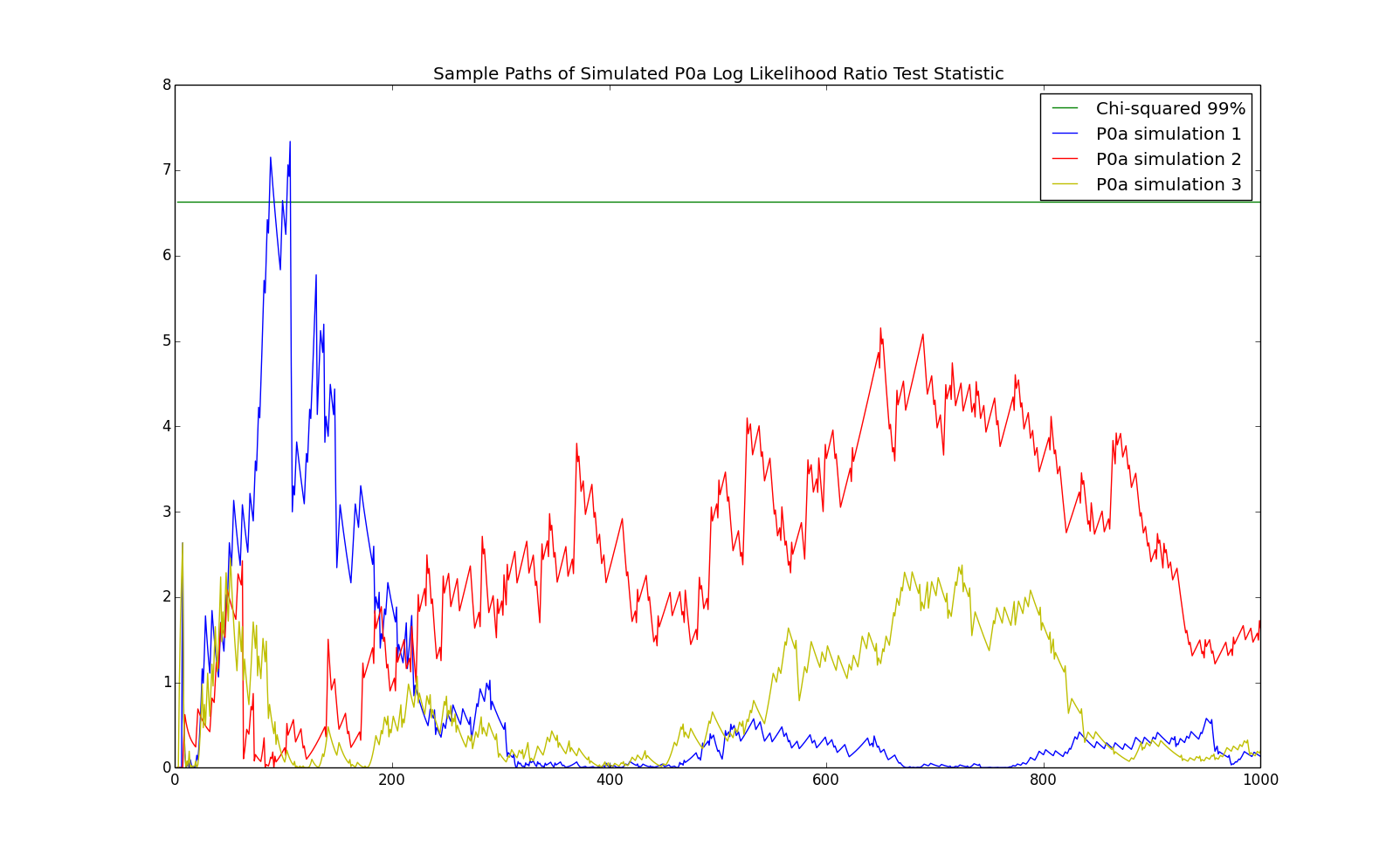
The previous theorem says that the log likelihood ratio is asymptotically $\chi^2$ distributed. However, this doesn't tell us how many observations are required in order to accurately calculate the probability of a the log likelihood ratio being as high as it is. In this section, we see how many observations are required for an IID versus first order Markov test. In particular, we simulate consider a the IID process with state space $\left\{0,1\right\}$ and probabilities: \begin{eqnarray*} p = \left(\begin{array}{cc}p_0 & p_1\end{array}\right) = \left(\begin{array}{cc}0.75 & 0.25\end{array}\right) \end{eqnarray*} We will refer to this model as P0a, as it is a $0$th order Markov chain and it is the first one (hence, the 'a'). We simulate observations of length $1,000$ from this process and calculate the log likelihood ratio between a first order Markov chain and an IID process: \begin{eqnarray*} \sum_{j=1}^m\sum_{k=1}^m n_{s_i,s_j}{\left(x^n\right)} \log \left(\frac{n_{s_i,s_j}{\left(x^n\right)}\sum_{i=1}^m\sum_{j=1}^m n_{s_i,s_j}{\left(x^n\right)}}{\sum_{j=1}^m n_{s_i,s_j}{\left(x^n\right)}\sum_{i=1}^m n_{s_i,s_j}{\left(x^n\right)}}\right) \end{eqnarray*} Note that the first order Markov chain has $m*(m-1) = 2$ parameters and the IID model has $m-1 = 1$ parameter. Hence, the likelihood ratio test has $1$ degree of freedom. We then calculate whether the $99\%$ percentile of the $\chi^2$ distribution with $1$ degree of freedom: $6.635$. The chart below shows a few simulated sample paths of the log likelihood ratio test statistic along with the $6.635$ line:

An observation which the test indicates is first order Markov but which is really IID is called a false positive. Asymptotically, the probability of a false positive at the chosen level of $6.635$ is $1\%$. We repeat the above experiment $100,000$ times to see how well the asymptotic formula works. The results are demonstrated in the following chart.

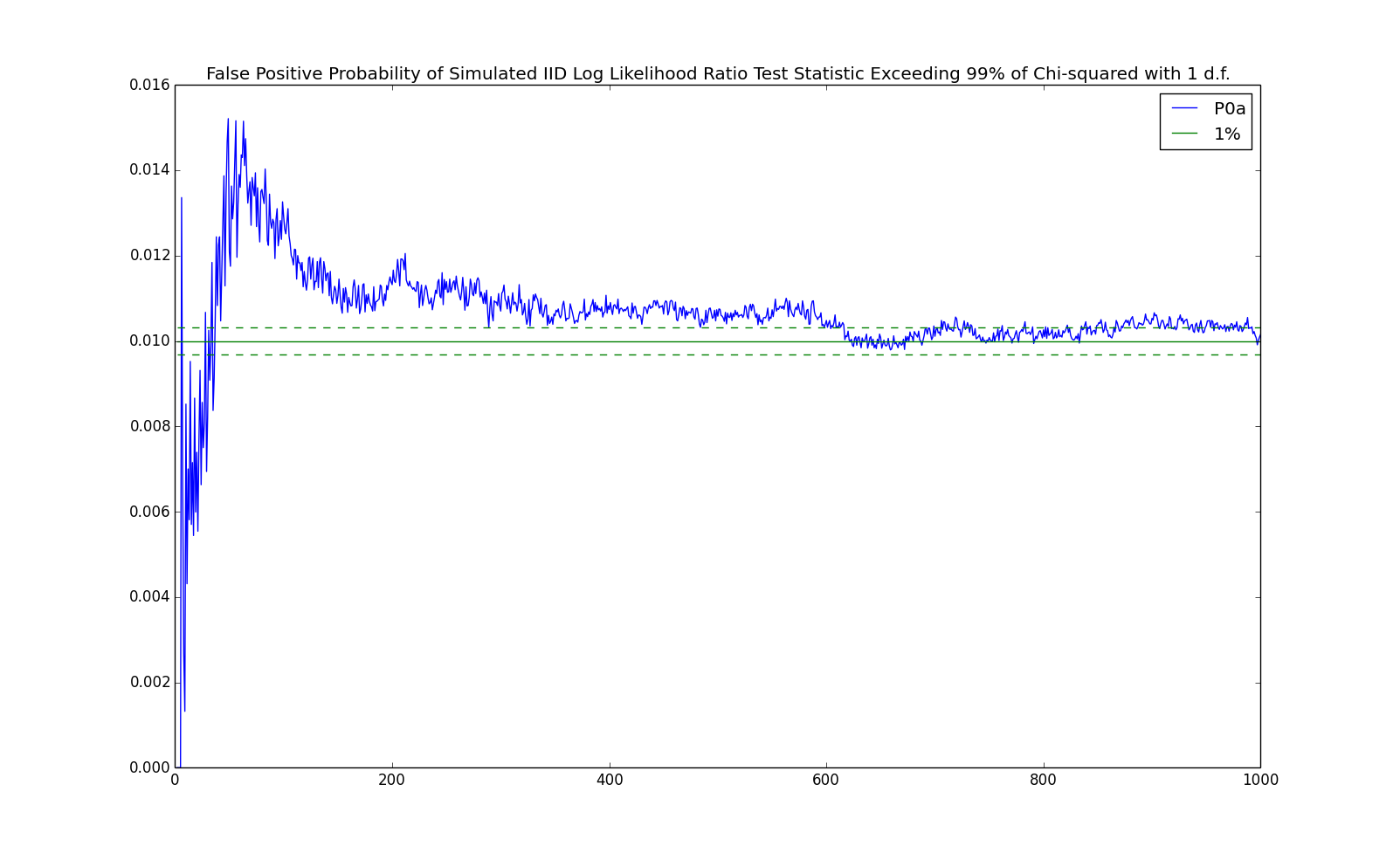
The blue line in the chart shows the percentage of samples which had a test statistic above the threshold level of $6.635$. The solid green line in the chart show the $1\%$ level. The dashed green lines show one standard deviation off of $1\%$ for this number of samples ($100,000$). From the chart, one can see that the asymptotic probability is accurate after a few hundred observations.

First order Markov process

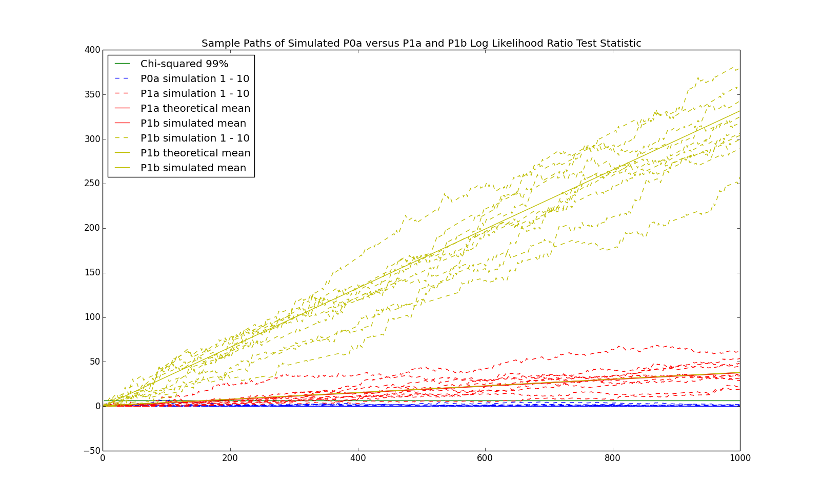
We now investigate the log likelihood ratio test with a first order Markov chain as the true process. We begin with the process with the following transition probabilities: \begin{eqnarray*} P = \left(\begin{array}{cc} p_{0,0} & p_{0,1}\\ p_{1,0} & p_{1,1}\\ \end{array}\right) = \left(\begin{array}{cc} 0.8 & 0.2\\ 0.6 & 0.4\\ \end{array}\right) \end{eqnarray*} which we refer to as P1a, as it is a $1$st order Markov chain and it is the first one (hence, the 'a'). Notice that the stationary distribution is given by: \begin{eqnarray*} \pi = \left(\begin{array}{cc}\frac{p_{1,0}}{p_{1,0}+p_{0,1}} & \frac{p_{0,1}}{p_{1,0}+p_{0,1}}\end{array}\right) = \left(\begin{array}{cc} 0.75 & 0.25\end{array}\right) \end{eqnarray*} which is exactly the model P0a discussed previously. Hence, the $0$th order Markov chain corresponding to this model is P0a. We now compare sample paths from P1a with sample paths from P0a:

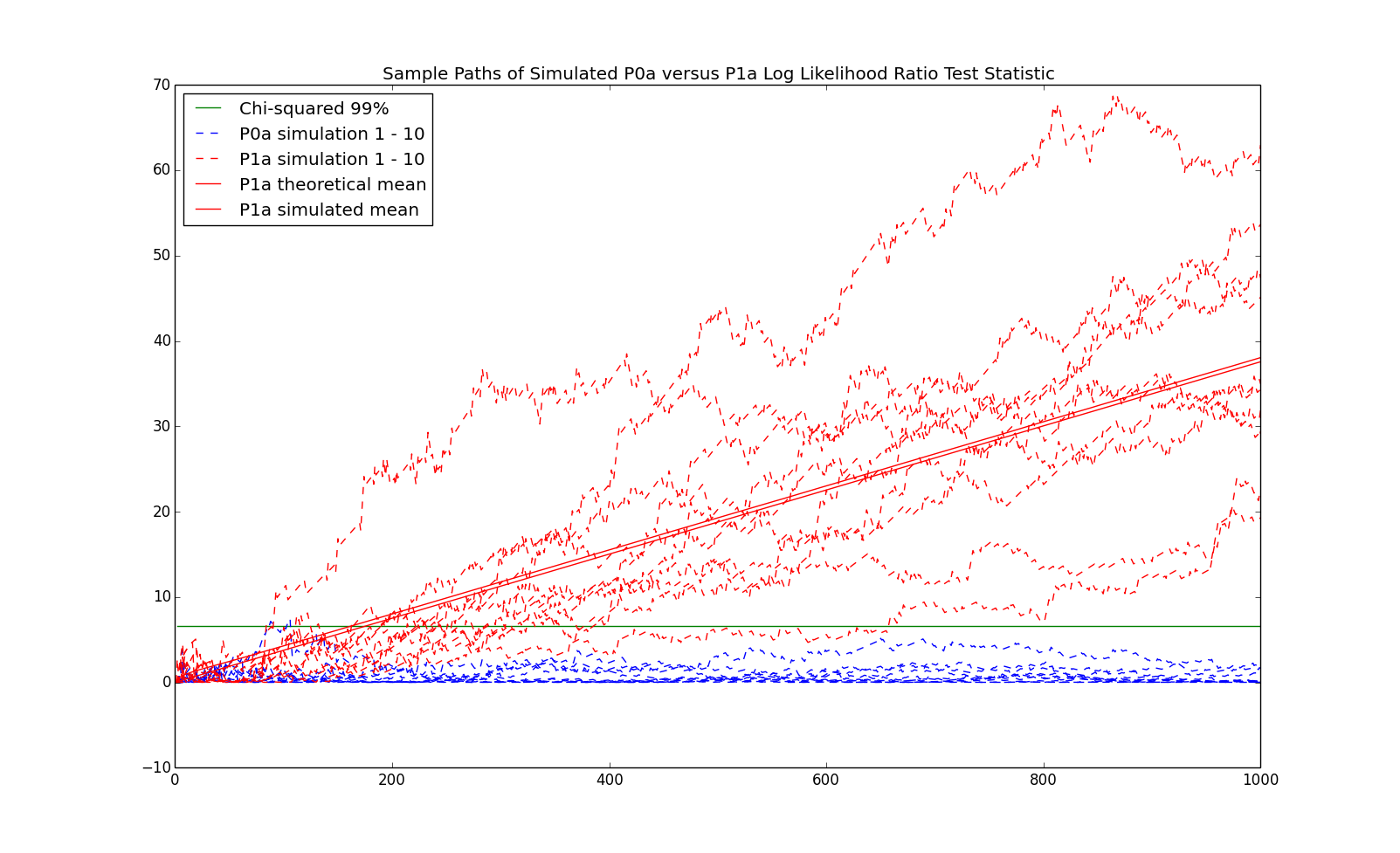
Note that the Kullback-Leibler distance between P1a and P0a is: \begin{eqnarray*} \sum_{i=1}^m \sum_{j=1}^m \pi_i p_{i,j} \log\left(\frac{p_{i,j}}{\pi_i}\right) \approx 0.0188 \end{eqnarray*} One of the solid red lines in the previous chart represented $2n$ times the Kullback-Leibler distance ($2$ since the test statistic is twice the log likelihood ratio test and $n$ from the approximate calculation of the log likelihood in equation (\ref{eq:KL})). The other solid red line represents the average of $100,000$ simulations.

The next chart shows the false negative rate, that is, the probability that we misclassify a first order Markov chain as a IID process for P1a along with the previously shown false positive rate:

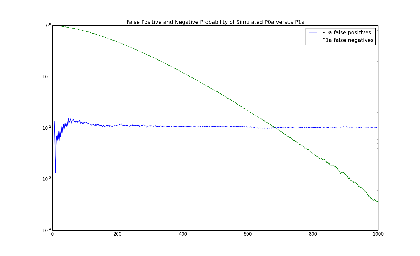
For this Markov chain, it seems to take about $500$ observations to reliably detect that the process is a first order Markov chain. However, this is dependent upon the Kullback-Leibler distance between the model and its stationary distribution. We now consider the following model which is further away: \begin{eqnarray*} P = \left(\begin{array}{cc} p_{0,0} & p_{0,1}\\ p_{1,0} & p_{1,1}\\ \end{array}\right) = \left(\begin{array}{cc} 0.9 & 0.1\\ 0.3 & 0.7\\ \end{array}\right) \end{eqnarray*} We refer to this model as P1b. The stationary distribution is still P0a, that is $\pi = \left(\begin{array}{cc}0.75 & 0.25\end{array}\right)$. The Kullback-Leibler distance is now $\approx 0.166$, approximately $9$ times as big as P1a. The sample paths of the log likelihood ratio test are demonstrated in the following chart:

and the false positive and negative rates are demonstrated in the following chart:

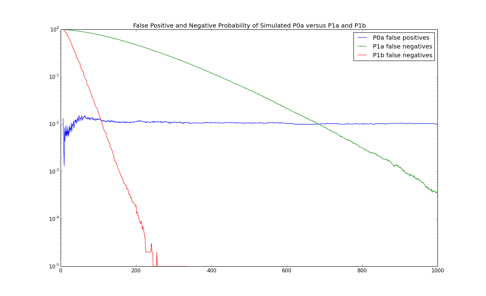
Since the Kullback-Leibler distance is larger, the order of P1b is deteced after less than $200$ observations compared with more than $500$ observations for P1a.

Second order Markov process

We now perform some simulations on an example of a second order Markov chain for which the stationary distribution on pairs is IID. We will introduce a second order Markov chain on the state space $\left\{0,1\right\}$. While the Markov chain is second order, we will present it as a first order Markov chain on the state space of pairs, since matrices are easier to present than $3$ dimensional objects: \begin{eqnarray*} P = \left(\begin{array}{cccc} p_{00,0} & p_{00,1} & 0 & 0\\ 0 & 0 & p_{01,0} & p_{01,1}\\ p_{10,0} & p_{10,1} & 0 & 0\\ 0 & 0 & p_{11,0} & p_{11,1}\\ \end{array}\right) = \left(\begin{array}{cccc} 0.8 & 0.2 & 0 & 0\\ 0 & 0 & 0.9 & 0.1\\ 0.6 & 0.4 & 0 & 0\\ 0 & 0 & 0.3 & 0.7\\ \end{array}\right) \end{eqnarray*} The stationary distribution is: \begin{eqnarray*} \pi = \left(\begin{array}{cccc}\pi_{0,0} & \pi_{0,1} & \pi_{1,0} & \pi_{1,1}\end{array}\right) = \left(\begin{array}{cccc}0.5625 & 0.1875 & 0.1875 & 0.0625\end{array}\right) \end{eqnarray*} From this, the first order Markov chain is given by: \begin{eqnarray*} \frac{\pi_{0,0}}{\pi_{0,0} + \pi_{0,1}} = \frac{0.5625}{0.5625+0.1875} = 0.75 = \frac{0.1875}{0.1875+0.0625} = \frac{\pi_{1,0}}{\pi_{1,0}+\pi_{1,1}} \end{eqnarray*} In other words, the probability of $0$ (and hence $1$) is independent of the previous state and is the same as P0a. Some sample paths of the log likelihood ratio test statistic between $0$th and $1$st order are given below:

The simulated false positive probability between $0$th and $1$st order are given below:

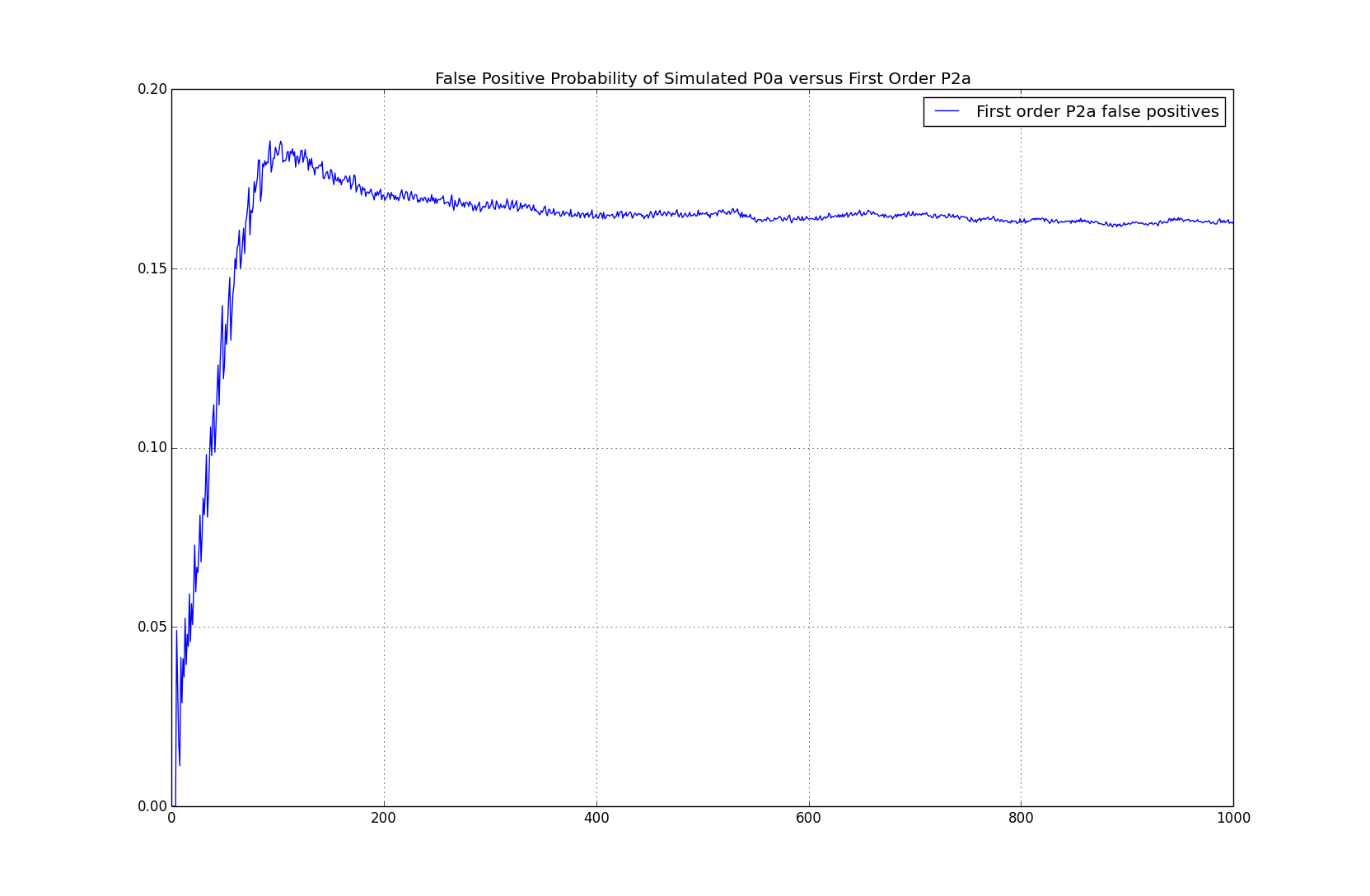
In this case, while the ultimate $2$nd order statistics (e.g. $n_{i,j}{\left(x^n\right)}$) which are used in the maximum likelihood estimator of the first order model, don't have any first order dependence, the process is still being detected as first order about $16\%$ of the time. Note that the result on the asymptotic distribution of the log likelihood ratio test doesn't hold here since the true model isn't $0$th order.

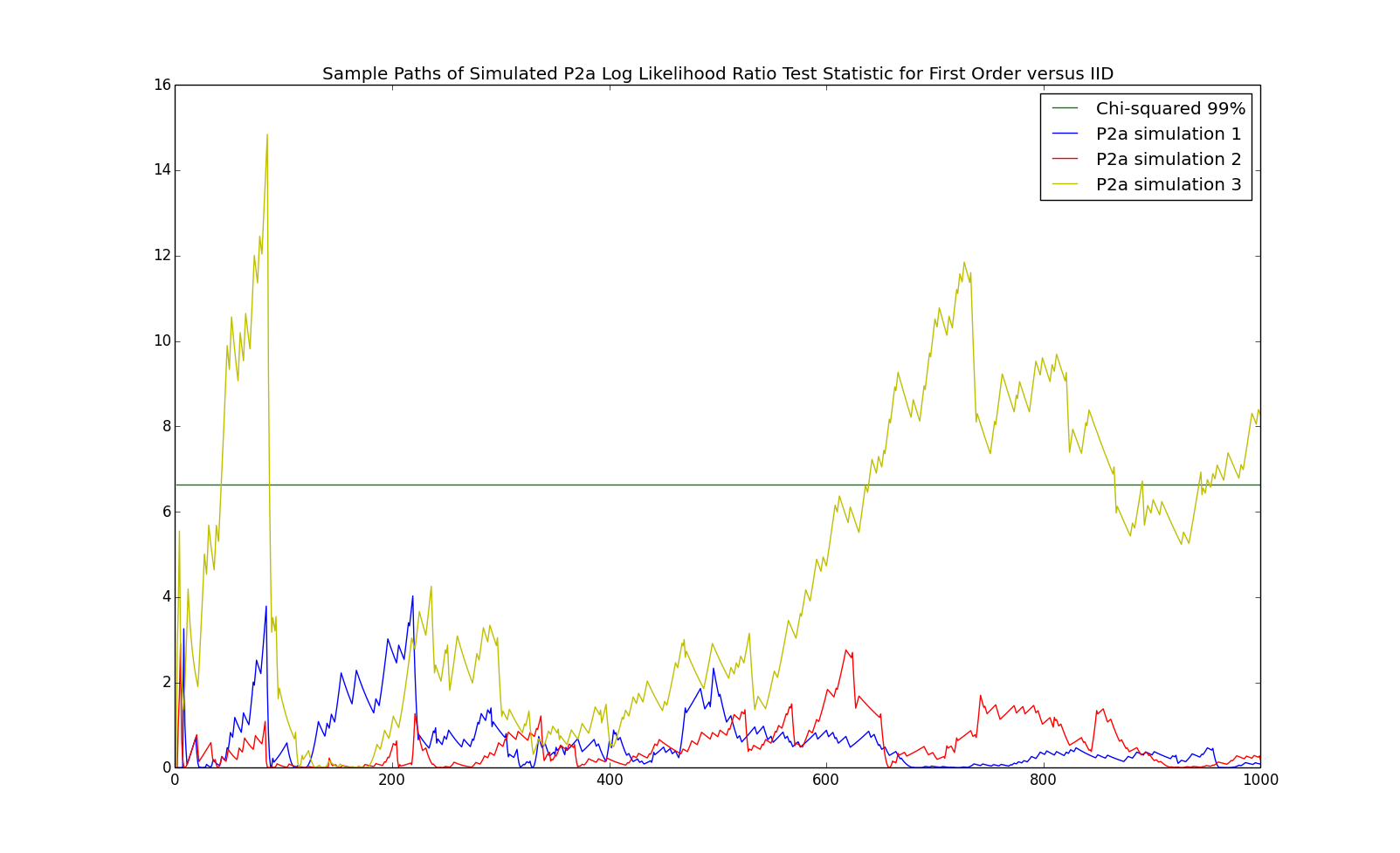
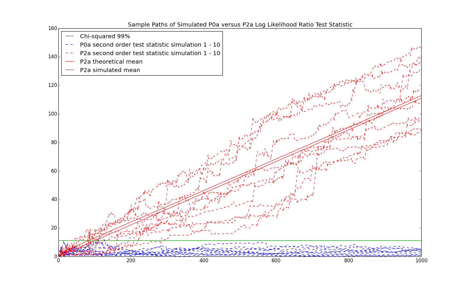
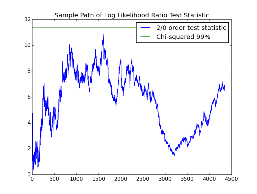
Finally, we present the test of $2$nd order versus $0$th order. In this case, the number of degrees of freedom is $m^2*(m-1) = 4$ parameters for the second order chain versus $m-1=1$ parameters for the IID process. The $\chi^2$ $99\%$ quantile with $3$ degrees of freedom is about $11.3$. Some sample paths of the test statistc from P2a as well as P0a are given below:

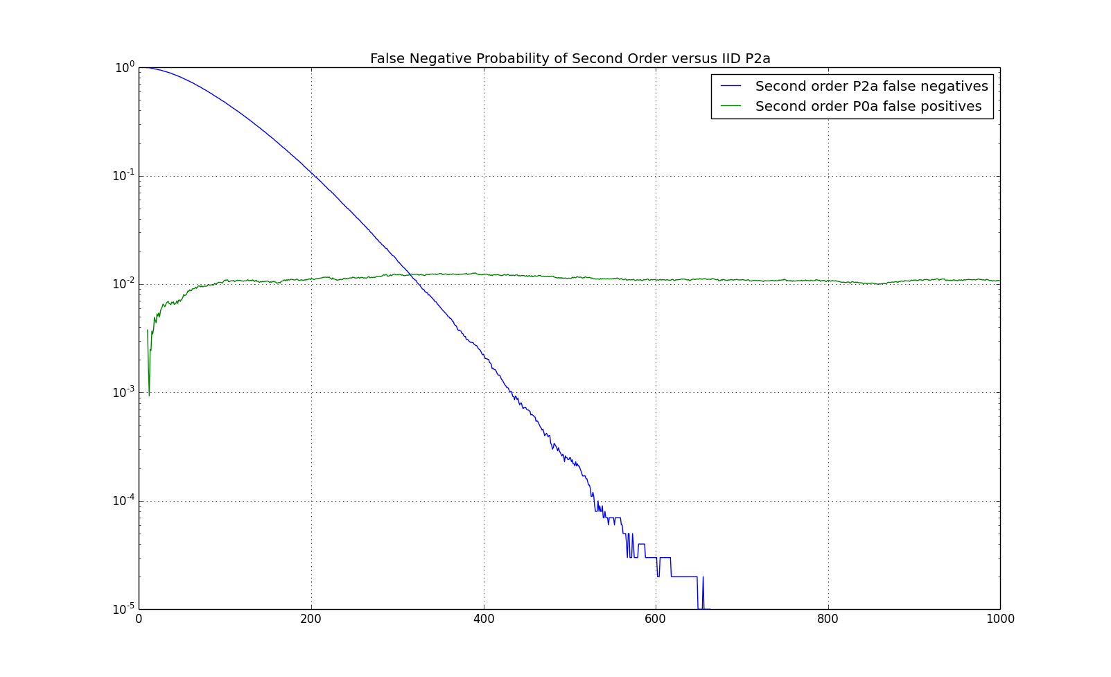
The simulated false negative probability between $0$th and $2$nd order for P2a and false positive probability for Pare given below:

Examples Trained on SPY Data

We now investigate data on the SPY ETF using Markov chains. We have downloaded daily data on SPY from Yahoo finance since the beginning of the year $2000$ (decimalization began in $1999$ which changed the way many stocks traded) through early $2017$ for a total of $4,348$ data points. Since stocks tend to grow over time, stock time series are non-stationary. For example, SPY went from and adjusted close of $\$105.37$ in the beginning of $2000$ to $\$232.51$ in mid April of $2017$. In order to eliminate the nonstationarity, we first transform the data into log returns: \begin{eqnarray*} r_t = \log\left(\frac{a_t}{a_{t-1}}\right) \end{eqnarray*} Note that log returns still may not be stationary but slow growth in value translates to a positive mean in returns. Log returns have a range of $(-\infty,\infty)$ as opposed to $[-1,\infty)$ for (arithmetic) returns and are also additive: the log return over multiple periods is the sum of the log returns over the individual periods.

Up/down model

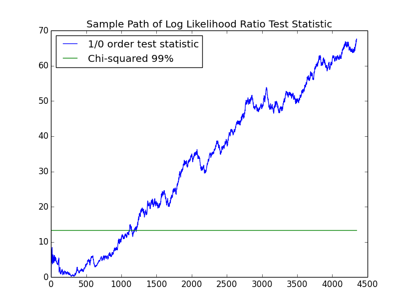
In order to encode the returns discretely, so that they can be fit with a Markov chain, we start by encoding them with "up" for positive returns and "down" for nonpositive returns. $53.8\%$ of the returns are positive. The following chart shows the evolution of the log likelihood ratio test between a $1$st and $0$th order Markov chain. Since there are $m*(m-1)=2$ parameters in the $1$st order model and $m-1=1$ in the $1$st order model, there is $1$ degree of freedom.

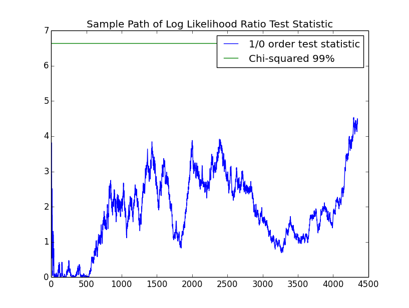
Unlike the simulations, in life, we usually only get a single sample path. For this path, we cannot reject the hypothesis that the process is IID with the $99\%$ confidence that we have been using.

As discussed, the $2$nd order model can still be significant against the $0$th order model even when the $1$st order model isn't. The next chart shows the log likelihood ratio of the $2$nd order model to the $0$th order model. Since there are $m^2*(m-1)=4$ parameters in the $2$nd order model and $m-1=1$ in the $1$st order model, there is $3$ degrees of freedom.

Again, we can not reject the IID hypothesis.

Since the $2$ state model that we trust is the IID model, we provide the maximum likelihood estimator of the model: \begin{eqnarray*} p \approx \left(\begin{array}{c}0.46 & 0.54\end{array}\right) \end{eqnarray*}

Up/down/flat model

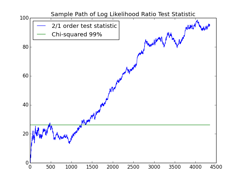
We now consider assigning $3$ discrete levels to the returns: up, down and flat. In order to choose the levels, we sort all the returns and choose the $33\frac{1}{3}$ and $66\frac{2}{3}$ percentiles. These turn out to be approximately $-25$bps and $38$bps. Note that this is cheating slightly: we are looking ahead in the data in order to choose the discretization. I generally prefer statistical methods which, at any given point in time, only use the data up to that point. However, looking ahead for this purpose is unlikely to dramatically skew the results. Any return less than $-25bps$ is labeled as down, greater than $38$bps, up, and in-between the two, flat. The following chart shows the log likelihood ratio between the $1$st and $0$th order models. In this case the $1$st order model has $m*(m-1)=6$ parameters and the $0$th order model has $m-1=2$ parameters so that the test has $4$ degrees of freedom.

Notice that the test statistic significantly exceeds the $99\%$ confidence level required to reject the IID hypothesis. Also, the curve shows the upward trend which is characteristic of the Kullback-Leibler distance being positive. The maximum likelihood estimator of the $0$th and $1$st order chains are given by: \begin{eqnarray*} P \approx \left(\begin{array}{ccc} 0.34 & 0.26 & 0.40\\ 0.33 & 0.38 & 0.29\\ 0.33 & 0.36 & 0.31\\ \end{array}\right) \end{eqnarray*} Recall that we have specifically chosen the boundaries of the states so that they have an equal probability of $\frac{1}{3}$ in the IID model. The $1$st order chain will differ from the $0$th order chain in so far as its probabilities are different. The most stand out probability in the $1$st order chain is the upper right corner probaiblity of $0.40$. This is the probability of going up given that the market has just gone down. This matches the phenomenon referred to by practitioners as dead cat bounce. Note that this probability is taken away from the probability of being flat. The probability of being flat when the market has just gone down is small.

In some ways it is not surprising that the more obvious $2$-state chain shows no structure: it is frequently looked at. If someone finds such regularity, that could give them a system to trade. In fact, such predictability in a $2$-state chain for stocks was pointed out in a paper in the Journal of Finance, the top finance journal, in 1991.

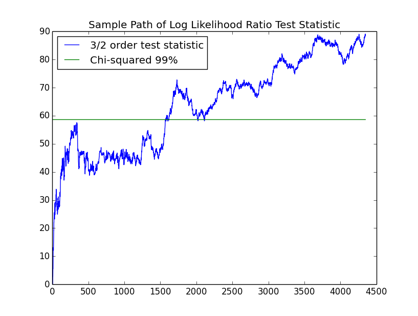
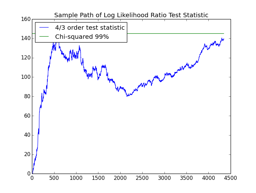
We now investigate whether the first order chain can be rejected for the second order chain. The second order chain has $m^2*(m-1)=18$ parameters versus $m*(m-1)=6$ for the first order chain so that the test has $12$ degrees of freedom. The chart follows:

The second order chain is also significant, though the slope of the path seems lower. The third order chain has $m^3*(m-1)=54$ parameters compared with $18$ for the second order chain. Hence, the test for the third order chain has $36$ degrees of freedom:

This is also significant but with even less of an upward trend in the path. The fourth order chain has $m^4*(m-1)=162$ parameters compared with $54$ for the third order chain making for $108$ degrees of freedom:

Thus, the fourth order process with $162$ parameters is not significant. We do not present the full details of the higher order chains here but point out a few highlights. The highest probability in the second order chain is the probability of staying flat given that you were flat and then up at about $0.48$. I'm not convinced that this is a real phenomenon. This is also borne out in the third order chain where the highest probability is the probability of staying flat after going up and being flat for the two prior periods at about $0.55$. Roughly speaking, the phenomenon seems to be that the market goes back to flat after going up if it is in a "flat regime". The next highest probability in the third order chain is the probability of going up after $3$ consecutive down periods at $0.49$. This is again the dead cat bounce.

It is possible to consider variable length Markov chains which have higher order for some transitions. The same technique used here: the log likelihood ratio test can be applied to this model. For example, it would be interesting to explore how many transitions this dead cat bounce phenomenon continues, that is, how many down days does in a row before the probability of an up day stops increasing and reaches a stable level. It would be helpful to do this without increasing the number of parameters for non-significant transitions. If someone wants to pursue variable length Markov chains as a project, please see me.

References

A good reference for statistical theory for Markov chains is:

Billingsley, Patrick. Statistical Inference for Markov Processes. The University of Chicago Press. 1961.

For the law of large numbers for Markov chains, see Theorem 4.2.1 of:

Kemeny, John G. and Snell, J. Laurie. Finite Markov Chains, chapter IV. Springer, 1960.

Note that they use the term "ergodic" for what I'm calling "irreducible". Both terms are generally used in the literature. The material presented here is scattered throughout several chapters.