Convergence in MCMC
As mentioned, MCMC, in particular the Metropolis Hastings algorithm, will always converge to the posterior distribution. However, how long it takes to converge is uncertain. We construct a (somewhat artificial) example demonstrating this. Suppose the posterior that we wish to construct is a $\beta$ distribution with parameters $\alpha$ and $1$. We wish to use MCMC to calculate the expected value of the posterior distribution whose value can be calculated analytically: \begin{eqnarray*} \int x \frac{\Gamma(\alpha+1)}{\Gamma(\alpha)\Gamma(1)} x^{\alpha-1} dx = \int \alpha x^{\alpha} dx = \frac{\alpha}{1+\alpha} \end{eqnarray*} We will use the proposal distribution be $\beta$ with parameters $1+\alpha$ and $1$. Notice that, unlike most cases, the proposal distribution is not dependent upon $x$. We now calculate the acceptance probability, $\rho$: \begin{eqnarray*} \rho = \min\left(1,\frac{f(y) q(x|y)}{f(x) q(y|x)}\right) = \min\left(1,\frac{\alpha y^{\alpha-1} \frac{1}{1+\alpha}x^\alpha}{\alpha x^{\alpha-1} \frac{1}{1+\alpha}y^\alpha}\right) = \min\left(1,\frac{x}{y}\right) \end{eqnarray*} We pick a $y$ from the proposal distribution and then replace $x$ with that $y$ randomly with probability $\rho$.
First, we look at the convergence when $\alpha=1$:
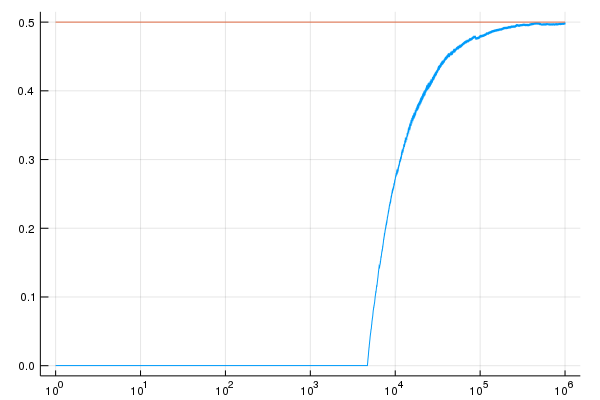 There is an interesting phenomenon which has occured here.
It turns out that we randomly chose an initial value of $x$ and were very unlucky in our choice happened to be about $0.00018$.
Since, $\rho$ is at most $\frac{x}{y}$, it will be some time (in this case 4,701 iterations) until we choose a $y$ small enough that it is likely to be accepted.
However, after 78,329 iterations, we no longer see any errors worse than $5\%$.
The chart below shows the same study with a different (more typical) random seed:
There is an interesting phenomenon which has occured here.
It turns out that we randomly chose an initial value of $x$ and were very unlucky in our choice happened to be about $0.00018$.
Since, $\rho$ is at most $\frac{x}{y}$, it will be some time (in this case 4,701 iterations) until we choose a $y$ small enough that it is likely to be accepted.
However, after 78,329 iterations, we no longer see any errors worse than $5\%$.
The chart below shows the same study with a different (more typical) random seed:
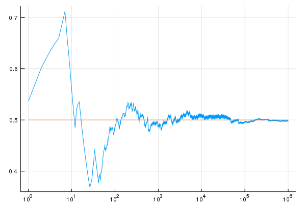
In this case, after 294 iterations, we no longer see any errors worse than $5\%$.
Now we consider the case where $\alpha=0.1$. The covergence of the expected value is given below:
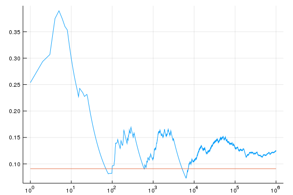
Notice that, even after 1,000,000 iterations, the error is still over $37\%$.
Note that this example is somewhat artificial. For example, when we looked at the problem of binomial trials with a $\beta$ prior, we found that the posterior value of the $\alpha$ parameter corresponds to the number of observations implied by the posterior (some equivalent observations from the prior and some actual observations). Since the problem above occurs when $\alpha=0.1$, it corresponds with no actual observations. In some more realistic examples, it is possible to show slow convergence as well. In either case, one has to quesiton whether convergence has been achieved.
There are several areas of practice and research in this direction:
- Many practitioners use diagnostics, typically by running multiple instances of the same MCMC chain and comparing the results across chains.
- Several researchers have attempted to find the speed of convergence of MCMC and related techniques. While there have been some results in this area, the theory is well behind the practice and the theoretical results tend not to apply to specific problems that not pragamatically oriented.
- There is a Markov chain simulation technique called Coupling from the Past which, when it stops, is guarenteed to be in the stationary distribution of the Markov chain. Note that the techique doesn't stop at a fixed time step.
Random Functions
Consider a set of functions $\left\{f_1, f_2, \ldots, f_k\right\}$ from a set $S = \left\{s_1, s_2, \ldots, s_m\right\}$ into itself, $f_i:S\rightarrow S$. Consider the process, $X_1, X_2, \ldots$ generated as follows:
- Choose $X_1$ randomly according to some distribution $\pi$ on $S$.
-
For each $t\ge 1$:
- Choose a function, $F_t$, randomly from $\left\{f_1,f_2,\ldots,f_k\right\}$ with probabilities $p_1, p_2, \ldots, p_k$ independently.
- Let $X_{t+1} = F_k\left(X_t\right)$.
We make a few remarks on random functions:
- It turns out that, not only are random function as described above Markov chains but also, every Markov chain can be represented by random functions.
- If we make the probabilities of which function to choose at each step dependent upon the state, the process is still a Markov chain.
Doubly Stochastic Matrices
A matrix, $P\in\mathbb{R}^{m\times m}$, is doubly stochastic if it is non-negative and has both row sums and column sums equal to $1$: \begin{eqnarray*} P_{i,j} & \ge & 0 \mbox{ for $i\in\left\{1,\ldots,m\right\}$, $j\in\left\{1,\ldots,m\right\}$}\\ \sum_{i=1}^m P_{i,j} & = & 1 \mbox{ for $j\in\left\{1,\ldots,m\right\}$}\\ \sum_{j=1}^m P_{i,j} & = & 1 \mbox{ for $i\in\left\{1,\ldots,m\right\}$}\\ \end{eqnarray*}
Every doubly stochastic matrix has the uniform distribution, $\pi_i = \frac{1}{m}$ as a stationary distribution: \begin{eqnarray*} \sum_{i=1}^m \pi_i P_{i,j} = \sum_{i=1}^m \frac{1}{m} P_{i,j} = \frac{1}{m} \sum_{i=1}^m P_{i,j} = \frac{1}{m} = \pi_j \end{eqnarray*} Similarly, every transition matrix which has the uniform distribution as a stationary distribution is doubly stochastic: \begin{eqnarray*} \sum_{i=1}^m P_{i,j} = \sum_{i=1}^m m \frac{1}{m} P_{i,j} = m \sum_{i=1}^m \pi_i P_{i,j} = m \pi_j = m \frac{1}{m} = 1 \end{eqnarray*}
A famous theorem of Birkhoff gives us a representation of doubly stochastic matrices. A permutation is a function $f$ from a finite set into the same set which has the following properties:
- One-to-one: if $f(x) = f(y)$ then $x=y$.
- Onto: for all $y$ there is an $x$ such that $f(x) = y$.
Every doubly stochastic matrix is a convex combination of permutation matrices, that is, for any doubly stochastic matrix $Q$, there are permutation matrices $P_1, P_2, \ldots, P_k$ and nonnegative weights $\lambda_1, \lambda_2, \ldots, \lambda_k$ with $\sum_{i=1}^k \lambda_k=1$ such that: \begin{eqnarray*} Q = \sum_{i=1}^k \lambda_i P_i \end{eqnarray*}
Since permutations are functions, doubly stochastic matrices are random functions when the functions are permutations.Reversible Markov Chains
In this section, we will explore reversible Markov chains. One statement of the Markovian property is that the past and future are independent given the present. This statement is symmetric in time: reversing time would leave the statement unchanged. However, for an aperiodic irreducible Markov chain which starts at a single state, over time it converges to a stationary distribution and not vice versa. This asymmetry will not occur if we start in the stationary distribution.
Also, note that our definition of time was infinite in the forward direction but not in the backward direction: we assume a Markov chain starts at time $1$ and goes on infinitely. In order to discuss reversing time for a Markov chain, we either need to make time infinite in both directions or talk about a finite segment of time. We'll choose the latter:
Let $X_1, X_2, \ldots, X_n$ is an irreducible homogeneous Markov chain with transition matrix $P$ and initial distribution equal to the stationary distribution, $\pi$. If $Y_i = X_{n-i}$, then $Y_1, Y_2, \ldots, Y_n$ is a homogeneous Markov chain with transition matrix $\tilde{P}$ satisfying the following relation: \begin{eqnarray}\label{reverse} \pi_i \tilde{P}_{i,j} = \pi_jP_{j,i} \end{eqnarray}
Note that (\ref{reverse}) is symmetric with respect to $P$ and $\tilde{P}$. In other words, the reverse Markov chain of the reverse Markov chain is the original Markov chain. We now go through some examples.
Example: A Birth-Death Process
We consider a birth-death process. Let the states of the Markov chain be $\{1,\ldots,m\}$. Let $p$ be the probability of going up from each state and $q$ the probability of going down. Hence, the transition matrix is given by: \begin{eqnarray*} P = \left(\begin{array}{ccccccccc} 1-p & p & 0 & 0 & \ldots & 0 & 0 & 0 & 0\\ q & 1-p-q & p & 0 & \ldots & 0 & 0 & 0 & 0\\ 0 & q & 1-p-q & p & \ldots & 0 & 0 & 0 & 0\\ \ldots & \ldots & \ldots & \ldots & \ldots & \ldots & \ldots & \ldots & \ldots\\ 0 & 0 & 0 & 0 & \ldots & q & 1-p-q & p & 0\\ 0 & 0 & 0 & 0 & \ldots & 0 & q & 1-p-q & p\\ 0 & 0 & 0 & 0 & \ldots & 0 & 0 & q & 1-q\\ \end{array}\right) \end{eqnarray*} We can use the Markov chain tree theorem to find that the stationary distribution is given by: \begin{eqnarray*} \pi_i = \frac{p^{i-1}q^{m-i}}{\sum_{i=1}^m p^{i-1}q^{m-i}} \end{eqnarray*} Solving the equation (\ref{reverse}), we get: \begin{eqnarray*} \tilde{P}_{i,j} = P_{j,i}\frac{\pi_j}{\pi_i} \end{eqnarray*} so that: \begin{eqnarray*} \tilde{P}_{i,i+1} = P_{i+1,i}\frac{\pi_{i+1}}{\pi_i} = q\frac{\frac{p^iq^{m-i-1}}{\sum_{i=1}^m p^{i-1}q^{m-i}}}{\frac{p^{i-1}q^{m-i}}{\sum_{i=1}^m p^{i-1}q^{m-i}}} = q\frac{p^iq^{m-i-1}}{p^{i-1}q^{m-i}} = q\frac{p}{q} = p \end{eqnarray*} and: \begin{eqnarray*} \tilde{P}_{i+1,i} = P_{i,i+1}\frac{\pi_i}{\pi_{i+1}} = p\frac{\frac{p^{i-1}q^{m-i}}{\sum_{i=1}^m p^{i-1}q^{m-i}}}{\frac{p^iq^{m-i-1}}{\sum_{i=1}^m p^{i-1}q^{m-i}}} = q\frac{p^{i-1}q^{m-i}}{p^iq^{m-i-1}} = p\frac{q}{p} = q \end{eqnarray*} From this, it can be concluded that the transition matrix of the reversed birth-death process is the same as the transition matrix of the original birth-death process. Note that this is the case for every irreducible birth-death process, not just the process mentioned here.
Example: A Regime-switching Model
As mentioned in the previous example, for an irreducible birth-death process, the reverse Markov chain is the same as the original Markov chain. The $3$-state regime-switching model is a birth-death process. In this example, we find the reversal of the $4$-state regime-switching model. The transition probability matrix is given by: \begin{eqnarray*} P \approx \left(\begin{array}{cccc} 0.9508 & 0.0492 & 0.0000 & 0.0000\\ 0.0070 & 0.9766 & 0.0164 & 0.0000\\ 0.0004 & 0.0099 & 0.9475 & 0.0422\\ 0.0000 & 0.0000 & 0.0375 & 0.9625\\ \end{array}\right) \end{eqnarray*} and the stationary distribution is given by: \begin{eqnarray*} \pi \approx \left(\begin{array}{cccc} 0.0342 & 0.2203 & 0.3508 & 0.3947\\ \end{array}\right) \end{eqnarray*} The reverse Markov chain is then given by: \begin{eqnarray*} \left(\begin{array}{cccc} 0.9508 & 0.0451 & 0.0041 & 0.0000\\ 0.0076 & 0.9766 & 0.0158 & 0.0000\\ 0.0000 & 0.0103 & 0.9475 & 0.0422\\ 0.0000 & 0.0000 & 0.0375 & 0.9625\\ \end{array}\right) \end{eqnarray*} Note that, unlike the previous example, $\tilde{P}\ne P$. For example, $\tilde{P}_{1,2} = 0.0451 \ne 0.0492 = P_{1,2}$. A few observations:
- The diagonals of $\tilde{P}$ and $P$ are equivalent since: \begin{eqnarray*} \tilde{P}_{i,i} = \frac{P_{i,i}\pi_i}{\pi_i} = P_{i,i} \end{eqnarray*} Hence, this will always be the case.
- The pattern of $0$'s in $\tilde{P}$ is the transpose of the pattern of $0$'s in $P$ since if $P_{i,j} = 0$ then: \begin{eqnarray*} \tilde{P}_{j,i} = \frac{P_{i,j}\pi_i}{\pi_j} = 0 \end{eqnarray*} By duality, if $\tilde{P}_{i,j}=0$ then $P_{j,i} = 0$.
-
Norris, J. R.. Markov Chains. Cambridge University Press, 1999..
This is a good general book on Markov chains. Our discussion of reversibility is taken largely from this book.
Example: An Absorbing Chain
We now consider the reverse of mortgage default model so that we can see what goes wrong when the Markov chain is not irreducible. Let $P$ be the transition matrix and $X_1, X_2, \ldots, X_n$ be a sample path from this Markov chain with initial distribution such that $X_1=C$. Let $Y_i = X_{n-i+1}$. \begin{eqnarray*} \mathbb{P}\left(Y_{i+1}=D\right|\left.Y_i=D\right) & = & \frac{\mathbb{P}\left(Y_{i+1}=D, Y_i=D\right)}{\mathbb{P}\left(Y_i=D\right)}\\ & = & \frac{\mathbb{P}\left(X_{n-i}=D, X_{n-i+1}=D\right)}{\mathbb{P}\left(X_{n-i+1}=D\right)}\\ & = & \frac{P^{n-i-1}_{C,D}}{P^{n-i}_{C,D}}\\ & = & \frac{P^{n-i-1}_{C,D}}{P^{n-i-1}_{C,D} + P^{n-i-1}_{C,60}P_{60,D}}\\ \end{eqnarray*} This quantity is, in general, not constant with respect to $i$ so that $Y$ is not a homogeneous Markov chain.
In the first example above, the reverse Markov chain is the same as the original Markov chain. We refer to a Markov chain for which this is true as reversible. From (\ref{reverse}), we see that this is true when: \begin{eqnarray*} \pi_i P_{i,j} = \pi_j P_{j,i} \end{eqnarray*} This condition is known as the detailed balance condition. We point out another interpretation of it: \begin{eqnarray*} \mathbb{P}\left(X_1=i, X_2=j\right) = \mathbb{P}\left(X_2=j\right|\left. X_1=i\right)\mathbb{P}\left(X_1=i\right) = \pi_i P_{i,j} \end{eqnarray*} Hence, detailed balance holds if and only if: \begin{eqnarray*} \mathbb{P}\left(X_1=i, X_2=j\right) = \mathbb{P}\left(X_1=j, X_2=i\right) \end{eqnarray*} In other words, a Markov chain is reversible if and only if the matrix of joint probabilities is symmetric.
Symmetric Markov Chains
As mentioned, a Markov chain is reversible if the matrix of joint probabilities is symmetric. In this section, we explore what happens when the transition probability matrix is symmetric. First, note that such a symmetric stochastic matrix is doubly stochastic: \begin{eqnarray*} \sum_{i=1}^m P_{i,j} = \sum_{i=1}^m P_{j,i} = 1 \end{eqnarray*} Furthermore, it is reversible detailed balance holds with $\pi_i=\frac{1}{m}$: \begin{eqnarray*} \frac{1}{m} P_{i,j} = \frac{1}{m} P_{j,i} \end{eqnarray*} Furthermore, every reversible, doubly stochastic matrix is symmetric.